Section 5: More Theory & Practice
Section 5: More Theory & Practice
In this section, we delve into some of the deeper theory of estimation and hypothesis testing, including:
- finding statistics that are sufficient for a parameter
- defining the power of a hypothesis test
- determining the sample size necessary for conducting a "powerful" hypothesis test
- investigating the properties a "good" hypothesis test should possess
- defining and deriving likelihood ratio tests
We also get some practice on choosing an appropriate statistical method for analyzing a given set of data.
Lesson 24: Sufficient Statistics
Lesson 24: Sufficient StatisticsOverview
In the lesson on Point Estimation, we derived estimators of various parameters using two methods, namely, the method of maximum likelihood and the method of moments. The estimators resulting from these two methods are typically intuitive estimators. It makes sense, for example, that we would want to use the sample mean \(\bar{X}\) and sample variance \(S^2\) to estimate the mean \(\mu\) and variance \(\sigma^2\) of a normal population.
In the process of estimating such a parameter, we summarize, or reduce, the information in a sample of size \(n\), \(X_1, X_2,\ldots, X_n\), to a single number, such as the sample mean \(\bar{X}\). The actual sample values are no longer important to us. That is, if we use a sample mean of 3 to estimate the population mean \(\mu\), it doesn't matter if the original data values were (1, 3, 5) or (2, 3, 4). Has this process of reducing the \(n\) data points to a single number retained all of the information about \(\mu\) that was contained in the original \(n\) data points? Or has some information about the parameter been lost through the process of summarizing the data? In this lesson, we'll learn how to find statistics that summarize all of the information in a sample about the desired parameter. Such statistics are called sufficient statistics, and hence the name of this lesson.
Objectives
- To learn a formal definition of sufficiency.
- To learn how to apply the Factorization Theorem to identify a sufficient statistic.
- To learn how to apply the Exponential Criterion to identify a sufficient statistic.
- To extend the definition of sufficiency for one parameter to two (or more) parameters.
24.1 - Definition of Sufficiency
24.1 - Definition of SufficiencySufficiency is the kind of topic in which it is probably best to just jump right in and state its definition. Let's do that!
- Sufficient
-
Let \(X_1, X_2, \ldots, X_n\) be a random sample from a probability distribution with unknown parameter \(\theta\). Then, the statistic:
\(Y = u(X_1, X_2, ... , X_n) \)
is said to be sufficient for \(\theta\) if the conditional distribution of \(X_1, X_2, \ldots, X_n\), given the statistic \(Y\), does not depend on the parameter \(\theta\).
Example 24-1

Let \(X_1, X_2, \ldots, X_n\) be a random sample of \(n\) Bernoulli trials in which:
- \(X_i=1\) if the \(i^{th}\) subject likes Pepsi
- \(X_i=0\) if the \(i^{th}\) subject does not like Pepsi
If \(p\) is the probability that subject \(i\) likes Pepsi, for \(i = 1, 2,\ldots,n\), then:
- \(X_i=1\) with probability \(p\)
- \(X_i=0\) with probability \(q = 1 − p\)
Suppose, in a random sample of \(n=40\) people, that \(Y = \sum_{i=1}^{n}X_i =22\) people like Pepsi. If we know the value of \(Y\), the number of successes in \(n\) trials, can we gain any further information about the parameter \(p\) by considering other functions of the data \(X_1, X_2, \ldots, X_n\)? That is, is \(Y\) sufficient for \(p\)?
Answer
The definition of sufficiency tells us that if the conditional distribution of \(X_1, X_2, \ldots, X_n\), given the statistic \(Y\), does not depend on \(p\), then \(Y\) is a sufficient statistic for \(p\). The conditional distribution of \(X_1, X_2, \ldots, X_n\), given \(Y\), is by definition:
\(P(X_1 = x_1, ... , X_n = x_n |Y = y) = \dfrac{P(X_1 = x_1, ... , X_n = x_n, Y = y)}{P(Y=y)}\) (**)
Now, for the sake of concreteness, suppose we were to observe a random sample of size \(n=3\) in which \(x_1=1, x_2=0, \text{ and }x_3=1\). In this case:
\( P(X_1 = 1, X_2 = 0, X_3 =1, Y=1)=0\)
because the sum of the data values, \( \sum_{i=1}^{n}X_i \), is 1 + 0 + 1 = 2, but \(Y\), which is defined to be the sum of the \(X_i\)'s is 1. That is, because \(2\ne 1\), the event in the numerator of the starred (**) equation is an impossible event and therefore its probability is 0.
Now, let's consider an event that is possible, namely ( \(X_1=1, X_2=0, X_3=1, Y=2\)). In that case, we have, by independence:
\( P(X_1 = 1, X_2 = 0, X_3 =1, Y=2) = p(1-p) p=p^2(1-p)\)
So, in general:
\(P(X_1 = x_1, X_2 = x_2, ... , X_n = x_n, Y = y) = 0 \text{ if } \sum_{i=1}^{n}x_i \ne y \)
and:
\(P(X_1 = x_1, X_2 = x_2, ... , X_n = x_n, Y = y) = p^y(1-p)^{n-y} \text{ if } \sum_{i=1}^{n}x_i = y \)
Now, the denominator in the starred (**) equation above is the binomial probability of getting exactly \(y\) successes in \(n\) trials with a probability of success \(p\). That is, the denominator is:
\( P(Y=y) = \binom{n}{y} p^y(1-p)^{n-y}\)
for \(y = 0, 1, 2,\ldots, n\). Putting the numerator and denominator together, we get, if \(y=0, 1, 2, \ldots, n\), that the conditional probability is:
\(P(X_1 = x_1, ... , X_n = x_n |Y = y) = \dfrac{p^y(1-p)^{n-y}}{\binom{n}{y} p^y(1-p)^{n-y}} =\dfrac{1}{\binom{n}{y}} \text{ if } \sum_{i=1}^{n}x_i = y\)
and:
\(P(X_1 = x_1, ... , X_n = x_n |Y = y) = 0 \text{ if } \sum_{i=1}^{n}x_i \ne y \)
Aha! We have just shown that the conditional distribution of \(X_1, X_2, \ldots, X_n\) given \(Y\) does not depend on \(p\). Therefore, \(Y\) is indeed sufficient for \(p\). That is, once the value of \(Y\) is known, no other function of \(X_1, X_2, \ldots, X_n\) will provide any additional information about the possible value of \(p\).
24.2 - Factorization Theorem
24.2 - Factorization TheoremWhile the definition of sufficiency provided on the previous page may make sense intuitively, it is not always all that easy to find the conditional distribution of \(X_1, X_2, \ldots, X_n\) given \(Y\). Not to mention that we'd have to find the conditional distribution of \(X_1, X_2, \ldots, X_n\) given \(Y\) for every \(Y\) that we'd want to consider a possible sufficient statistic! Therefore, using the formal definition of sufficiency as a way of identifying a sufficient statistic for a parameter \(\theta\) can often be a daunting road to follow. Thankfully, a theorem often referred to as the Factorization Theorem provides an easier alternative! We state it here without proof.
- Factorization
-
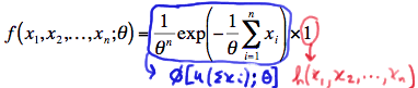
Let \(X_1, X_2, \ldots, X_n\) denote random variables with joint probability density function or joint probability mass function \(f(x_1, x_2, \ldots, x_n; \theta)\), which depends on the parameter \(\theta\). Then, the statistic \(Y = u(X_1, X_2, ... , X_n) \) is sufficient for \(\theta\) if and only if the p.d.f (or p.m.f.) can be factored into two components, that is:
\(f(x_1, x_2, ... , x_n;\theta) = \phi [ u(x_1, x_2, ... , x_n);\theta ] h(x_1, x_2, ... , x_n) \)
where:
- \(\phi\) is a function that depends on the data \(x_1, x_2, \ldots, x_n\) only through the function \(u(x_1, x_2, \ldots, x_n)\), and
- the function \(h((x_1, x_2, \ldots, x_n)\) does not depend on the parameter \(\theta\)
Let's put the theorem to work on a few examples!
Example 24-2

Let \(X_1, X_2, \ldots, X_n\) denote a random sample from a Poisson distribution with parameter \(\lambda>0\). Find a sufficient statistic for the parameter \(\lambda\).
Answer
Because \(X_1, X_2, \ldots, X_n\) is a random sample, the joint probability mass function of \(X_1, X_2, \ldots, X_n\) is, by independence:
\(f(x_1, x_2, ... , x_n;\lambda) = f(x_1;\lambda) \times f(x_2;\lambda) \times ... \times f(x_n;\lambda)\)
Inserting what we know to be the probability mass function of a Poisson random variable with parameter \(\lambda\), the joint p.m.f. is therefore:
\(f(x_1, x_2, ... , x_n;\lambda) = \dfrac{e^{-\lambda}\lambda^{x_1}}{x_1!} \times\dfrac{e^{-\lambda}\lambda^{x_2}}{x_2!} \times ... \times \dfrac{e^{-\lambda}\lambda^{x_n}}{x_n!}\)
Now, simplifying, by adding up all \(n\) of the \(\lambda\)s in the exponents, as well as all \(n\) of the \(x_i\)'s in the exponents, we get:
\(f(x_1, x_2, ... , x_n;\lambda) = \left(e^{-n\lambda}\lambda^{\Sigma x_i} \right) \times \left( \dfrac{1}{x_1! x_2! ... x_n!} \right)\)
Hey, look at that! We just factored the joint p.m.f. into two functions, one (\(\phi\)) being only a function of the statistic \(Y=\sum_{i=1}^{n}X_i\) and the other (h) not depending on the parameter \(\lambda\):
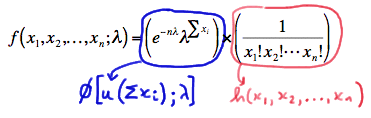
Therefore, the Factorization Theorem tells us that \(Y=\sum_{i=1}^{n}X_i\) is a sufficient statistic for \(\lambda\). But, wait a second! We can also write the joint p.m.f. as:
\(f(x_1, x_2, ... , x_n;\lambda) = \left(e^{-n\lambda}\lambda^{n\bar{x}} \right) \times \left( \dfrac{1}{x_1! x_2! ... x_n!} \right)\)
Therefore, the Factorization Theorem tells us that \(Y = \bar{X}\) is also a sufficient statistic for \(\lambda\)!
If you think about it, it makes sense that \(Y = \bar{X}\) and \(Y=\sum_{i=1}^{n}X_i\) are both sufficient statistics, because if we know \(Y = \bar{X}\), we can easily find \(Y=\sum_{i=1}^{n}X_i\). And, if we know \(Y=\sum_{i=1}^{n}X_i\), we can easily find \(Y = \bar{X}\).
The previous example suggests that there can be more than one sufficient statistic for a parameter \(\theta\). In general, if \(Y\) is a sufficient statistic for a parameter \(\theta\), then every one-to-one function of \(Y\) not involving \(\theta\) is also a sufficient statistic for \(\theta\). Let's take a look at another example.
Example 24-3

Let \(X_1, X_2, \ldots, X_n\) be a random sample from a normal distribution with mean \(\mu\) and variance 1. Find a sufficient statistic for the parameter \(\mu\).
Answer
Because \(X_1, X_2, \ldots, X_n\) is a random sample, the joint probability density function of \(X_1, X_2, \ldots, X_n\) is, by independence:
\(f(x_1, x_2, ... , x_n;\mu) = f(x_1;\mu) \times f(x_2;\mu) \times ... \times f(x_n;\mu)\)
Inserting what we know to be the probability density function of a normal random variable with mean \(\mu\) and variance 1, the joint p.d.f. is:
\(f(x_1, x_2, ... , x_n;\mu) = \dfrac{1}{(2\pi)^{1/2}} exp \left[ -\dfrac{1}{2}(x_1 - \mu)^2 \right] \times \dfrac{1}{(2\pi)^{1/2}} exp \left[ -\dfrac{1}{2}(x_2 - \mu)^2 \right] \times ... \times \dfrac{1}{(2\pi)^{1/2}} exp \left[ -\dfrac{1}{2}(x_n - \mu)^2 \right] \)
Collecting like terms, we get:
\(f(x_1, x_2, ... , x_n;\mu) = \dfrac{1}{(2\pi)^{n/2}} exp \left[ -\dfrac{1}{2}\sum_{i=1}^{n}(x_i - \mu)^2 \right]\)
A trick to making the factoring of the joint p.d.f. an easier task is to add 0 to the quantity in parentheses in the summation. That is:
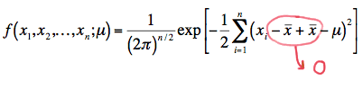
Now, squaring the quantity in parentheses, we get:
\(f(x_1, x_2, ... , x_n;\mu) = \dfrac{1}{(2\pi)^{n/2}} exp \left[ -\dfrac{1}{2}\sum_{i=1}^{n}\left[ (x_i - \bar{x})^2 +2(x_i - \bar{x}) (\bar{x}-\mu)+ (\bar{x}-\mu)^2\right] \right]\)
And then distributing the summation, we get:
\(f(x_1, x_2, ... , x_n;\mu) = \dfrac{1}{(2\pi)^{n/2}} exp \left[ -\dfrac{1}{2}\sum_{i=1}^{n} (x_i - \bar{x})^2 - (\bar{x}-\mu) \sum_{i=1}^{n}(x_i - \bar{x}) -\dfrac{1}{2}\sum_{i=1}^{n}(\bar{x}-\mu)^2\right] \)
But, the middle term in the exponent is 0, and the last term, because it doesn't depend on the index \(i\), can be added up \(n\) times:
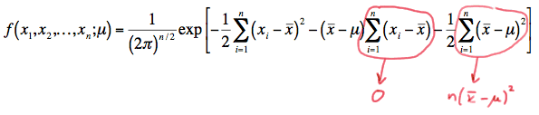
So, simplifying, we get:
\(f(x_1, x_2, ... , x_n;\mu) = \left\{ exp \left[ -\dfrac{n}{2} (\bar{x}-\mu)^2 \right] \right\} \times \left\{ \dfrac{1}{(2\pi)^{n/2}} exp \left[ -\dfrac{1}{2}\sum_{i=1}^{n} (x_i - \bar{x})^2 \right] \right\} \)
In summary, we have factored the joint p.d.f. into two functions, one (\(\phi\)) being only a function of the statistic \(Y = \bar{X}\) and the other (h) not depending on the parameter \(\mu\):
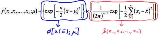
Therefore, the Factorization Theorem tells us that \(Y = \bar{X}\) is a sufficient statistic for \(\mu\). Now, \(Y = \bar{X}^3\) is also sufficient for \(\mu\), because if we are given the value of \( \bar{X}^3\), we can easily get the value of \(\bar{X}\) through the one-to-one function \(w=y^{1/3}\). That is:
\( W=(\bar{X}^3)^{1/3}=\bar{X} \)
On the other hand, \(Y = \bar{X}^2\) is not a sufficient statistic for \(\mu\), because it is not a one-to-one function. That is, if we are given the value of \(\bar{X}^2\), using the inverse function:
\(w=y^{1/2}\)
we get two possible values, namely:
\(-\bar{X}\) and \(+\bar{X}\)
We're getting so good at this, let's take a look at one more example!
Example 24-4
Let \(X_1, X_2, \ldots, X_n\) be a random sample from an exponential distribution with parameter \(\theta\). Find a sufficient statistic for the parameter \(\theta\).
Answer
Because \(X_1, X_2, \ldots, X_n\) is a random sample, the joint probability density function of \(X_1, X_2, \ldots, X_n\) is, by independence:
\(f(x_1, x_2, ... , x_n;\theta) = f(x_1;\theta) \times f(x_2;\theta) \times ... \times f(x_n;\theta)\)
Inserting what we know to be the probability density function of an exponential random variable with parameter \(\theta\), the joint p.d.f. is:
\(f(x_1, x_2, ... , x_n;\theta) =\dfrac{1}{\theta}exp\left( \dfrac{-x_1}{\theta}\right) \times \dfrac{1}{\theta}exp\left( \dfrac{-x_2}{\theta}\right) \times ... \times \dfrac{1}{\theta}exp\left( \dfrac{-x_n}{\theta} \right) \)
Now, simplifying, by adding up all \(n\) of the \(\theta\)s and the \(n\) \(x_i\)'s in the exponents, we get:
\(f(x_1, x_2, ... , x_n;\theta) =\dfrac{1}{\theta^n}exp\left( - \dfrac{1}{\theta} \sum_{i=1}^{n} x_i\right) \)
We have again factored the joint p.d.f. into two functions, one (\(\phi\)) being only a function of the statistic \(Y=\sum_{i=1}^{n}X_i\) and the other (h) not depending on the parameter \(\theta\):
Therefore, the Factorization Theorem tells us that \(Y=\sum_{i=1}^{n}X_i\) is a sufficient statistic for \(\theta\). And, since \(Y = \bar{X}\) is a one-to-one function of \(Y=\sum_{i=1}^{n}X_i\), it implies that \(Y = \bar{X}\) is also a sufficient statistic for \(\theta\).
24.3 - Exponential Form
24.3 - Exponential FormYou might not have noticed that in all of the examples we have considered so far in this lesson, every p.d.f. or p.m.f. could we written in what is often called exponential form, that is:
\( f(x;\theta) =exp\left[K(x)p(\theta) + S(x) + q(\theta) \right] \)
with
- \(K(x)\) and \(S(x)\) being functions only of \(x\),
- \(p(\theta)\) and \(q(\theta)\) being functions only of the parameter \(\theta\)
- The support being free of the parameter \(\theta\).
First, we had Bernoulli random variables with p.m.f. written in exponential form as:
with:
- \(K(x)\) and \(S(x)\) being functions only of \(x\),
- \(p(p)\) and \(q(p)\) being functions only of the parameter \(p\)
- The support \(x=0\), 1 not depending on the parameter \(p\)
Okay, we just skipped a lot of steps in that second equality sign, that is, in getting from point A (the typical p.m.f.) to point B (the p.m.f. written in exponential form). So, let's take a look at that more closely. We start with:
\( f(x;p) =p^x(1-p)^{1-x} \)
Is the p.m.f. in exponential form? Doesn't look like it to me! We clearly need an "exp" to appear up front. The only way we are going to get that without changing the underlying function is by taking the inverse function, that is, the natural log ("ln"), at the same time. Doing so, we get:
\( f(x;p) =exp\left[\text{ln}(p^x(1-p)^{1-x}) \right] \)
Is the p.m.f. now in exponential form? Nope, not yet, but at least it's looking more hopeful. All of the steps that follow now involve using what we know about the properties of logarithms. Recognizing that the natural log of a product is the sum of the natural logs, we get:
\( f(x;p) =exp\left[\text{ln}(p^x) + \text{ln}(1-p)^{1-x} \right] \)
Is the p.m.f. now in exponential form? Nope, still not yet, because \(K(x)\), \(p(p)\), \(S(x)\), and \(q(p)\) can't yet be identified as following exponential form, but we are certainly getting closer. Recognizing that the log of a power is the power times the log of the base, we get:
\( f(x;p) =exp\left[x\text{ln}(p) + (1-x)\text{ln}(1-p) \right] \)
This is getting tiring. Is the p.m.f. in exponential form yet? Nope, afraid not yet. Let's distribute that \((1-x)\) in that last term. Doing so, we get:
\( f(x;p) =exp\left[x\text{ln}(p) + \text{ln}(1-p) - x\text{ln}(1-p) \right] \)
Is the p.m.f. now in exponential form? Let's take a closer look. Well, in the first term, we can identify the \(K(x)p(p)\) and in the middle term, we see a function that depends only on the parameter \(p\):
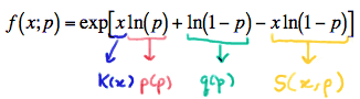
Now, all we need is the last term to depend only on \(x\) and we're as good as gold. Oh, rats! The last term depends on both \(x\) and \(p\). So back to work some more! Recognizing that the log of a quotient is the difference between the logs of the numerator and denominator, we get:
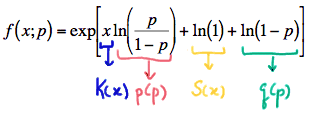
\( f(x;p) =exp\left[x\text{ln}\left( \frac{p}{1-p}\right) + \text{ln}(1-p) \right] \)
Is the p.m.f. now in exponential form? So close! Let's just add 0 in (by way of the natural log of 1) to make it obvious. Doing so, we get:
\( f(x;p) =exp\left[x\text{ln}\left( \frac{p}{1-p}\right) + \text{ln}(1) + \text{ln}(1-p) \right] \)
Yes, we have finally written the Bernoulli p.m.f. in exponential form:
Whew! So, we've fully explored writing the Bernoulli p.m.f. in exponential form! Let's get back to reviewing all of the p.m.f.'s we've encountered in this lesson. We had Poisson random variables whose p.m.f. can be written in exponential form as:
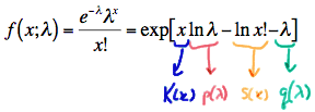
with
- \(K(x)\) and \(S(x)\) being functions only of \(x\),
- \(p(\lambda)\) and \(q(\lambda)\) being functions only of the parameter \(\lambda\)
- The support \(x = 0, 1, 2, \ldots\) not depending on the parameter \(\lambda\)
Then, we had \(N(\mu, 1)\) random variables whose p.d.f. can be written in exponential form as:
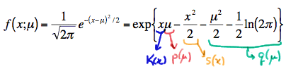
with
- \(K(x)\) and \(S(x)\) being functions only of \(x\),
- \(p(\mu)\) and \(q(\mu)\) being functions only of the parameter \(\mu\)
- The support \(-\infty<x<\infty\) not depending on the parameter \(\mu\)
Then, we had exponential random variables random variables whose p.d.f. can be written in exponential form as:
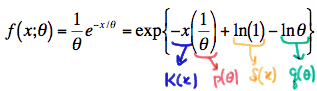
with
- \(K(x)\) and \(S(x)\) being functions only of \(x\),
- \(p(\theta)\) and \(q(\theta)\) being functions only of the parameter \(\theta\)
- The support \(x\ge 0\) not depending on the parameter \(\theta\).
Happily, it turns out that writing p.d.f.s and p.m.f.s in exponential form provides us yet a third way of identifying sufficient statistics for our parameters. The following theorem tells us how.
Exponential Criterion:
Let \(X_1, X_2, \ldots, X_n\) be a random sample from a distribution with a p.d.f. or p.m.f. of the exponential form:
\( f(x;\theta) =exp\left[K(x)p(\theta) + S(x) + q(\theta) \right] \)
with a support that does not depend on \(\theta\). Then, the statistic:
\( \sum_{i=1}^{n} K(X_i) \)
is sufficient for \(\theta\).
Proof
Because \(X_1, X_2, \ldots, X_n\) is a random sample, the joint p.d.f. (or joint p.m.f.) of \(X_1, X_2, \ldots, X_n\) is, by independence:
\(f(x_1, x_2, ... , x_n;\theta)= f(x_1;\theta) \times f(x_2;\theta) \times ... \times f(x_n;\theta) \)
Inserting what we know to be the p.m.f. or p.d.f. in exponential form, we get:
\(f(x_1, ... , x_n;\theta)=\text{exp}\left[K(x_1)p(\theta) + S(x_1)+q(\theta)\right] \times ... \times \text{exp}\left[K(x_n)p(\theta) + S(x_n)+q(\theta)\right] \)
Collecting like terms in the exponents, we get:
\(f(x_1, ... , x_n;\theta)=\text{exp}\left[p(\theta)\sum_{i=1}^{n}K(x_i) + \sum_{i=1}^{n}S(x_i) + nq(\theta)\right] \)
which can be factored as:
\(f(x_1, ... , x_n;\theta)=\left\{ \text{exp}\left[p(\theta)\sum_{i=1}^{n}K(x_i) + nq(\theta)\right]\right\} \times \left\{ \text{exp}\left[\sum_{i=1}^{n}S(x_i)\right] \right\} \)
We have factored the joint p.m.f. or p.d.f. into two functions, one (\(\phi\)) being only a function of the statistic \(Y=\sum_{i=1}^{n}K(X_i)\) and the other (h) not depending on the parameter \(\theta\):
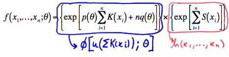
Therefore, the Factorization Theorem tells us that \(Y=\sum_{i=1}^{n}K(X_i)\) is a sufficient statistic for \(\theta\).
Let's try the Exponential Criterion out on an example.
Example 24-5

Let \(X_1, X_2, \ldots, X_n\) be a random sample from a geometric distribution with parameter \(p\). Find a sufficient statistic for the parameter \(p\).
Answer
The probability mass function of a geometric random variable is:
\(f(x;p) = (1-p)^{x-1}p\)
for \(x=1, 2, 3, \ldots\) The p.m.f. can be written in exponential form as:
\(f(x;p) = \text{exp}\left[ x\text{log}(1-p)+\text{log}(1)+\text{log}\left( \frac{p}{1-p} \right)\right] \)
Therefore, \(Y=\sum_{i=1}^{n}X_i\) is sufficient for \(p\). Easy as pie!
By the way, you might want to note that almost every p.m.f. or p.d.f. we encounter in this course can be written in exponential form. With that noted, you might want to make the Exponential Criterion the first tool you grab out of your toolbox when trying to find a sufficient statistic for a parameter.
24.4 - Two or More Parameters
24.4 - Two or More ParametersIn each of the examples we considered so far in this lesson, there is one and only one parameter. What happens if a probability distribution has two parameters, \(\theta_1\) and \(\theta_2\), say, for which we want to find sufficient statistics, \(Y_1\) and \(Y_2\)? Fortunately, the definitions of sufficiency can easily be extended to accommodate two (or more) parameters. Let's start by extending the Factorization Theorem.
- Definition (Factorization Theorem)
-
Let \(X_1, X_2, \ldots, X_n\) denote random variables with a joint p.d.f. (or joint p.m.f.):
\( f(x_1,x_2, ... ,x_n; \theta_1, \theta_2) \)
which depends on the parameters \(\theta_1\) and \(\theta_2\). Then, the statistics \(Y_1=u_1(X_1, X_2, ... , X_n)\) and \(Y_2=u_2(X_1, X_2, ... , X_n)\) are joint sufficient statistics for \(\theta_1\) and \(\theta_2\) if and only if:
\(f(x_1, x_2, ... , x_n;\theta_1, \theta_2) =\phi\left[u_1(x_1, ... , x_n), u_2(x_1, ... , x_n);\theta_1, \theta_2 \right] h(x_1, ... , x_n)\)
where:
- \(\phi\) is a function that depends on the data \((x_1, x_2, ... , x_n)\) only through the functions \(u_1(x_1, x_2, ... , x_n)\) and \(u_2(x_1, x_2, ... , x_n)\), and
- the function \(h(x_1, ... , x_n)\) does not depend on either of the parameters \(\theta_1\) or \(\theta_2\).
Let's try the extended theorem out for size on an example.
Example 24-6

Let \(X_1, X_2, \ldots, X_n\) denote a random sample from a normal distribution \(N(\theta_1, \theta_2\). That is, \(\theta_1\) denotes the mean \(\mu\) and \(\theta_2\) denotes the variance \(\sigma^2\). Use the Factorization Theorem to find joint sufficient statistics for \(\theta_1\) and \(\theta_2\).
Answer
Because \(X_1, X_2, \ldots, X_n\) is a random sample, the joint probability density function of \(X_1, X_2, \ldots, X_n\) is, by independence:
\(f(x_1, x_2, ... , x_n;\theta_1, \theta_2) = f(x_1;\theta_1, \theta_2) \times f(x_2;\theta_1, \theta_2) \times ... \times f(x_n;\theta_1, \theta_2) \times \)
Inserting what we know to be the probability density function of a normal random variable with mean \(\theta_1\) and variance \(\theta_2\), the joint p.d.f. is:
\(f(x_1, x_2, ... , x_n;\theta_1, \theta_2) = \dfrac{1}{\sqrt{2\pi\theta_2}} \text{exp} \left[-\dfrac{1}{2}\dfrac{(x_1-\theta_1)^2}{\theta_2} \right] \times ... \times = \dfrac{1}{\sqrt{2\pi\theta_2}} \text{exp} \left[-\dfrac{1}{2}\dfrac{(x_n-\theta_1)^2}{\theta_2} \right] \)
Simplifying by collecting like terms, we get:
\(f(x_1, x_2, ... , x_n;\theta_1, \theta_2) = \left(\dfrac{1}{\sqrt{2\pi\theta_2}}\right)^n \text{exp} \left[-\dfrac{1}{2}\dfrac{\sum_{i=1}^{n}(x_i-\theta_1)^2}{\theta_2} \right] \)
Rewriting the first factor, and squaring the quantity in parentheses, and distributing the summation, in the second factor, we get:
\(f(x_1, x_2, ... , x_n;\theta_1, \theta_2) = \text{exp} \left[\text{log}\left(\dfrac{1}{\sqrt{2\pi\theta_2}}\right)^n\right] \text{exp} \left[-\dfrac{1}{2\theta_2}\left\{ \sum_{i=1}^{n}x_{i}^{2} -2\theta_1\sum_{i=1}^{n}x_{i} +\sum_{i=1}^{n}\theta_{1}^{2} \right\}\right] \)
Simplifying yet more, we get:
\(f(x_1, x_2, ... , x_n;\theta_1, \theta_2) = \text{exp} \left[ -\dfrac{1}{2\theta_2}\sum_{i=1}^{n}x_{i}^{2}+\dfrac{\theta_1}{\theta_2}\sum_{i=1}^{n}x_{i} -\dfrac{n\theta_{1}^{2}}{2\theta_2}-n\text{log}\sqrt{2\pi\theta_2} \right]\)
Look at that! We have factored the joint p.d.f. into two functions, one (\(\phi\)) being only a function of the statistics \(Y_1=\sum_{i=1}^{n}X^{2}_{i}\) and \(Y_2=\sum_{i=1}^{n}X_i\), and the other (h) not depending on the parameters \(\theta_1\) and \(\theta_2\):
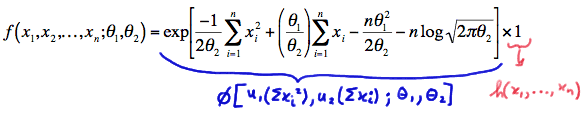
Therefore, the Factorization Theorem tells us that \(Y_1=\sum_{i=1}^{n}X^{2}_{i}\) and \(Y_2=\sum_{i=1}^{n}X_i\) are joint sufficient statistics for \(\theta_1\) and \(\theta_2\). And, the one-to-one functions of \(Y_1\) and \(Y_2\), namely:
\( \bar{X} =\dfrac{Y_2}{n}=\dfrac{1}{n}\sum_{i=1}^{n}X_i \)
and
\( S_2=\dfrac{Y_1-(Y_{2}^{2}/n)}{n-1}=\dfrac{1}{n-1} \left[\sum_{i=1}^{n}X_{i}^{2}-n\bar{X}^2 \right] \)
are also joint sufficient statistics for \(\theta_1\) and \(\theta_2\). Aha! We have just shown that the intuitive estimators of \(\mu\) and \(\sigma^2\) are also sufficient estimators. That is, the data contain no more information than the estimators \(\bar{X}\) and \(S^2\) do about the parameters \(\mu\) and \(\sigma^2\)! That seems like a good thing!
We have just extended the Factorization Theorem. Now, the Exponential Criterion can also be extended to accommodate two (or more) parameters. It is stated here without proof.
Exponential Criterion
Let \(X_1, X_2, \ldots, X_n\) be a random sample from a distribution with a p.d.f. or p.m.f. of the exponential form:
\( f(x;\theta_1,\theta_2)=\text{exp}\left[K_1(x)p_1(\theta_1,\theta_2)+K_2(x)p_2(\theta_1,\theta_2)+S(x) +q(\theta_1,\theta_2) \right] \)
with a support that does not depend on the parameters \(\theta_1\) and \(\theta_2\). Then, the statistics \(Y_1=\sum_{i=1}^{n}K_1(X_i)\) and \(Y_2=\sum_{i=1}^{n}K_2(X_i)\) are jointly sufficient for \(\theta_1\) and \(\theta_2\).
Let's try applying the extended exponential criterion to our previous example.
Example 24-6 continuted

Let \(X_1, X_2, \ldots, X_n\) denote a random sample from a normal distribution \(N(\theta_1, \theta_2)\). That is, \(\theta_1\) denotes the mean \(\mu\) and \(\theta_2\) denotes the variance \(\sigma^2\). Use the Exponential Criterion to find joint sufficient statistics for \(\theta_1\) and \(\theta_2\).
Answer
The probability density function of a normal random variable with mean \(\theta_1\) and variance \(\theta_2\) can be written in exponential form as:
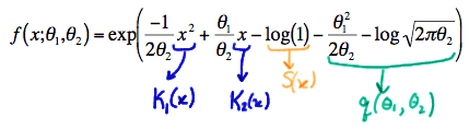
Therefore, the statistics \(Y_1=\sum_{i=1}^{n}X^{2}_{i}\) and \(Y_2=\sum_{i=1}^{n}X_i\) are joint sufficient statistics for \(\theta_1\) and \(\theta_2\).
Lesson 25: Power of a Statistical Test
Lesson 25: Power of a Statistical TestOverview
Whenever we conduct a hypothesis test, we'd like to make sure that it is a test of high quality. One way of quantifying the quality of a hypothesis test is to ensure that it is a "powerful" test. In this lesson, we'll learn what it means to have a powerful hypothesis test, as well as how we can determine the sample size n necessary to ensure that the hypothesis test we are conducting has high power.
25.1 - Definition of Power
25.1 - Definition of PowerLet's start our discussion of statistical power by recalling two definitions we learned when we first introduced to hypothesis testing:
- A Type I error occurs if we reject the null hypothesis \(H_0\) (in favor of the alternative hypothesis \(H_A\)) when the null hypothesis \(H_0\) is true. We denote \(\alpha=P(\text{Type I error})\).
- A Type II error occurs if we fail to reject the null hypothesis \(H_0\) when the alternative hypothesis \(H_A\) is true. We denote \(\beta=P(\text{Type II error})\).
You'll certainly need to know these two definitions inside and out, as you'll be thinking about them a lot in this lesson, and at any time in the future when you need to calculate a sample size either for yourself or for someone else.
Example 25-1

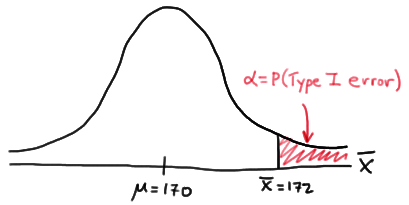
The Brinell hardness scale is one of several definitions used in the field of materials science to quantify the hardness of a piece of metal. The Brinell hardness measurement of a certain type of rebar used for reinforcing concrete and masonry structures was assumed to be normally distributed with a standard deviation of 10 kilograms of force per square millimeter. Using a random sample of \(n=25\) bars, an engineer is interested in performing the following hypothesis test:
- the null hypothesis \(H_0:\mu=170\)
- against the alternative hypothesis \(H_A:\mu>170\)
If the engineer decides to reject the null hypothesis if the sample mean is 172 or greater, that is, if \(\bar{X} \ge 172 \), what is the probability that the engineer commits a Type I error?
Answer
In this case, the engineer commits a Type I error if his observed sample mean falls in the rejection region, that is, if it is 172 or greater, when the true (unknown) population mean is indeed 170. Graphically, \(\alpha\), the engineer's probability of committing a Type I error looks like this:
Now, we can calculate the engineer's value of \(\alpha\) by making the transformation from a normal distribution with a mean of 170 and a standard deviation of 10 to that of \(Z\), the standard normal distribution using:
\(Z= \frac{\bar{X}-\mu}{\sigma / \sqrt{n}} \)
Doing so, we get:
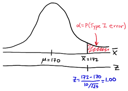
So, calculating the engineer's probability of committing a Type I error reduces to making a normal probability calculation. The probability is 0.1587 as illustrated here:
\(\alpha = P(\bar{X} \ge 172 \text { if } \mu = 170) = P(Z \ge 1.00) = 0.1587 \)
A probability of 0.1587 is a bit high. We'll learn in this lesson how the engineer could reduce his probability of committing a Type I error.
If, unknown to engineer, the true population mean were \(\mu=173\), what is the probability that the engineer commits a Type II error?
Answer
In this case, the engineer commits a Type II error if his observed sample mean does not fall in the rejection region, that is, if it is less than 172, when the true (unknown) population mean is 173. Graphically, \(\beta\), the engineer's probability of committing a Type II error looks like this:
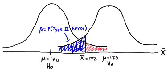
Again, we can calculate the engineer's value of \(\beta\) by making the transformation from a normal distribution with a mean of 173 and a standard deviation of 10 to that of \(Z\), the standard normal distribution. Doing so, we get:
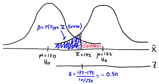
So, calculating the engineer's probability of committing a Type II error again reduces to making a normal probability calculation. The probability is 0.3085 as illustrated here:
\(\beta= P(\bar{X} < 172 \text { if } \mu = 173) = P(Z < -0.50) = 0.3085 \)
A probability of 0.3085 is a bit high. We'll learn in this lesson how the engineer could reduce his probability of committing a Type II error.
 If you think about it, considering the probability of committing a Type II error is quite similar to looking at a glass that is half empty. That is, rather than considering the probability that the engineer commits an error, perhaps we could consider the probability that the engineer makes the correct decision. Doing so, involves calculating what is called the power of the hypothesis test.
- Power of the Hypothesis Test
-
The power of a hypothesis test is the probability of making the correct decision if the alternative hypothesis is true. That is, the power of a hypothesis test is the probability of rejecting the null hypothesis \(H_0\) when the alternative hypothesis \(H_A\) is the hypothesis that is true.
Let's return to our engineer's problem to see if we can instead look at the glass as being half full!
Example 25-1 (continued)
If, unknown to the engineer, the true population mean were \(\mu=173\), what is the probability that the engineer makes the correct decision by rejecting the null hypothesis in favor of the alternative hypothesis?
Answer
In this case, the engineer makes the correct decision if his observed sample mean falls in the rejection region, that is, if it is greater than 172, when the true (unknown) population mean is 173. Graphically, the power of the engineer's hypothesis test looks like this:
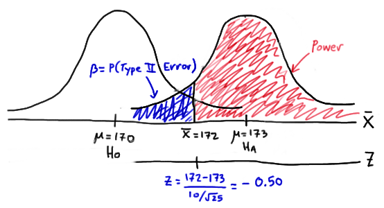
That makes the power of the engineer's hypothesis test 0.6915 as illustrated here:
\(\text{Power } = P(\bar{X} \ge 172 \text { if } \mu = 173) = P(Z \ge -0.50) = 0.6915 \)
which of course could have alternatively been calculated by simply subtracting the probability of committing a Type II error from 1, as shown here:
\(\text{Power } = 1 - \beta = 1 - 0.3085 = 0.6915 \)
At any rate, if the unknown population mean were 173, the engineer's hypothesis test would be at least a bit better than flipping a fair coin, in which he'd have but a 50% chance of choosing the correct hypothesis. In this case, he has a 69.15% chance. He could still do a bit better.
In general, for every hypothesis test that we conduct, we'll want to do the following:
-
Minimize the probability of committing a Type I error. That, is minimize \(\alpha=P(\text{Type I Error})\). Typically, a significance level of \(\alpha\le 0.10\) is desired.
-
Maximize the power (at a value of the parameter under the alternative hypothesis that is scientifically meaningful). Typically, we desire power to be 0.80 or greater. Alternatively, we could minimize \(\beta=P(\text{Type II Error})\), aiming for a type II error rate of 0.20 or less.
By the way, in the second point, what exactly does "at a value of the parameter under the alternative hypothesis that is scientifically meaningful" mean? Well, let's suppose that a medical researcher is interested in testing the null hypothesis that the mean total blood cholesterol in a population of patients is 200 mg/dl against the alternative hypothesis that the mean total blood cholesterol is greater than 200 mg/dl. Well, the alternative hypothesis contains an infinite number of possible values of the mean. Under the alternative hypothesis, the mean of the population could be, among other values, 201, 202, or 210. Suppose the medical researcher rejected the null hypothesis, because the mean was 201. Whoopdy-do...would that be a rocking conclusion? No, probably not. On the other hand, suppose the medical researcher rejected the null hypothesis, because the mean was 215. In that case, the mean is substantially different enough from the assumed mean under the null hypothesis, that we'd probably get excited about the result. In summary, in this example, we could probably all agree to consider a mean of 215 to be "scientifically meaningful," whereas we could not do the same for a mean of 201.
Now, of course, all of this talk is a bit if gibberish, because we'd never really know whether the true unknown population mean were 201 or 215, otherwise, we wouldn't have to be going through the process of conducting a hypothesis test about the mean. We can do something though. We can plan our scientific studies so that our hypothesis tests have enough power to reject the null hypothesis in favor of values of the parameter under the alternative hypothesis that are scientifically meaningful.
25.2 - Power Functions
25.2 - Power FunctionsExample 25-2

Let's take a look at another example that involves calculating the power of a hypothesis test.
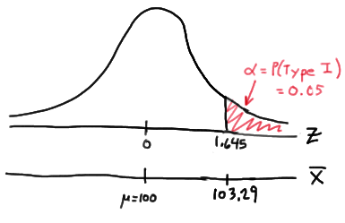
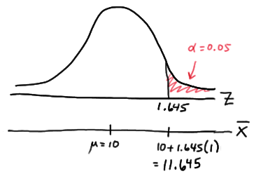
Let \(X\) denote the IQ of a randomly selected adult American. Assume, a bit unrealistically, that \(X\) is normally distributed with unknown mean \(\mu\) and standard deviation 16. Take a random sample of \(n=16\) students, so that, after setting the probability of committing a Type I error at \(\alpha=0.05\), we can test the null hypothesis \(H_0:\mu=100\) against the alternative hypothesis that \(H_A:\mu>100\).
What is the power of the hypothesis test if the true population mean were \(\mu=108\)?
Answer
Setting \(\alpha\), the probability of committing a Type I error, to 0.05, implies that we should reject the null hypothesis when the test statistic \(Z\ge 1.645\), or equivalently, when the observed sample mean is 106.58 or greater:

because we transform the test statistic \(Z\) to the sample mean by way of:
\(Z=\dfrac{\bar{X}-\mu}{\frac{\sigma}{\sqrt{n}}}\qquad \Rightarrow \bar{X}=\mu+Z\dfrac{\sigma}{\sqrt{n}} \qquad \bar{X}=100+1.645\left(\dfrac{16}{\sqrt{16}}\right)=106.58\)
Now, that implies that the power, that is, the probability of rejecting the null hypothesis, when \(\mu=108\) is 0.6406 as calculated here (recalling that \(Phi(z)\) is standard notation for the cumulative distribution function of the standard normal random variable):
\( \text{Power}=P(\bar{X}\ge 106.58\text{ when } \mu=108) = P\left(Z\ge \dfrac{106.58-108}{\frac{16}{\sqrt{16}}}\right) \\ = P(Z\ge -0.36)=1-P(Z<-0.36)=1-\Phi(-0.36)=1-0.3594=0.6406 \)
and illustrated here:
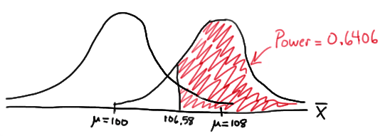
In summary, we have determined that we have (only) a 64.06% chance of rejecting the null hypothesis \(H_0:\mu=100\) in favor of the alternative hypothesis \(H_A:\mu>100\) if the true unknown population mean is in reality \(\mu=108\).
What is the power of the hypothesis test if the true population mean were \(\mu=112\)?
Answer
Because we are setting \(\alpha\), the probability of committing a Type I error, to 0.05, we again reject the null hypothesis when the test statistic \(Z\ge 1.645\), or equivalently, when the observed sample mean is 106.58 or greater. That means that the probability of rejecting the null hypothesis, when \(\mu=112\) is 0.9131 as calculated here:
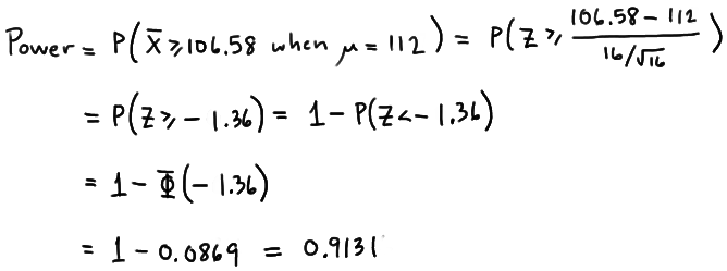
\( \text{Power}=P(\bar{X}\ge 106.58\text{ when }\mu=112)=P\left(Z\ge \frac{106.58-112}{\frac{16}{\sqrt{16}}}\right) \\ = P(Z\ge -1.36)=1-P(Z<-1.36)=1-\Phi(-1.36)=1-0.0869=0.9131 \)
and illustrated here:
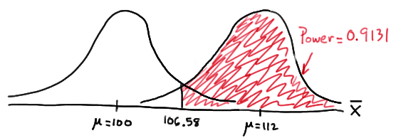
In summary, we have determined that we now have a 91.31% chance of rejecting the null hypothesis \(H_0:\mu=100\) in favor of the alternative hypothesis \(H_A:\mu>100\) if the true unknown population mean is in reality \(\mu=112\). Hmm.... it should make sense that the probability of rejecting the null hypothesis is larger for values of the mean, such as 112, that are far away from the assumed mean under the null hypothesis.
What is the power of the hypothesis test if the true population mean were \(\mu=116\)?
Answer
Again, because we are setting \(\alpha\), the probability of committing a Type I error, to 0.05, we reject the null hypothesis when the test statistic \(Z\ge 1.645\), or equivalently, when the observed sample mean is 106.58 or greater. That means that the probability of rejecting the null hypothesis, when \(\mu=116\) is 0.9909 as calculated here:

\(\text{Power}=P(\bar{X}\ge 106.58\text{ when }\mu=116) =P\left(Z\ge \dfrac{106.58-116}{\frac{16}{\sqrt{16}}}\right) = P(Z\ge -2.36)=1-P(Z<-2.36)= 1-\Phi(-2.36)=1-0.0091=0.9909 \)
and illustrated here:
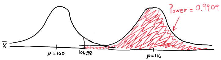
In summary, we have determined that, in this case, we have a 99.09% chance of rejecting the null hypothesis \(H_0:\mu=100\) in favor of the alternative hypothesis \(H_A:\mu>100\) if the true unknown population mean is in reality \(\mu=116\). The probability of rejecting the null hypothesis is the largest yet of those we calculated, because the mean, 116, is the farthest away from the assumed mean under the null hypothesis.
Are you growing weary of this? Let's summarize a few things we've learned from engaging in this exercise:
- First and foremost, my instructor can be tedious at times..... errrr, I mean, first and foremost, the power of a hypothesis test depends on the value of the parameter being investigated. In the above, example, the power of the hypothesis test depends on the value of the mean \(\mu\).
- As the actual mean \(\mu\) moves further away from the value of the mean \(\mu=100\) under the null hypothesis, the power of the hypothesis test increases.
It's that first point that leads us to what is called the power function of the hypothesis test. If you go back and take a look, you'll see that in each case our calculation of the power involved a step that looks like this:
\(\text{Power } =1 - \Phi (z) \) where \(z = \frac{106.58 - \mu}{16 / \sqrt{16}} \)
That is, if we use the standard notation \(K(\mu)\) to denote the power function, as it depends on \(\mu\), we have:
\(K(\mu) = 1- \Phi \left( \frac{106.58 - \mu}{16 / \sqrt{16}} \right) \)
So, the reality is your instructor could have been a whole lot more tedious by calculating the power for every possible value of \(\mu\) under the alternative hypothesis! What we can do instead is create a plot of the power function, with the mean \(\mu\) on the horizontal axis and the power \(K(\mu)\) on the vertical axis. Doing so, we get a plot in this case that looks like this:
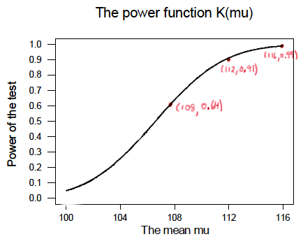
Now, what can we learn from this plot? Well:
-
We can see that \(\alpha\) (the probability of a Type I error), \(\beta\) (the probability of a Type II error), and \(K(\mu)\) are all represented on a power function plot, as illustrated here:
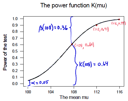
-
We can see that the probability of a Type I error is \(\alpha=K(100)=0.05\), that is, the probability of rejecting the null hypothesis when the null hypothesis is true is 0.05.
-
We can see the power of a test \(K(\mu)\), as well as the probability of a Type II error \(\beta(\mu)\), for each possible value of \(\mu\).
-
We can see that \(\beta(\mu)=1-K(\mu)\) and vice versa, that is, \(K(\mu)=1-\beta(\mu)\).
-
And we can see graphically that, indeed, as the actual mean \(\mu\) moves further away from the null mean \(\mu=100\), the power of the hypothesis test increases.
Now, what would do you suppose would happen to the power of our hypothesis test if we were to change our willingness to commit a Type I error? Would the power for a given value of \(\mu\) increase, decrease, or remain unchanged? Suppose, for example, that we wanted to set \(\alpha=0.01\) instead of \(\alpha=0.05\)? Let's return to our example to explore this question.
Example 25-2 (continued)

Let \(X\) denote the IQ of a randomly selected adult American. Assume, a bit unrealistically, that \(X\) is normally distributed with unknown mean \(\mu\) and standard deviation 16. Take a random sample of \(n=16\) students, so that, after setting the probability of committing a Type I error at \(\alpha=0.01\), we can test the null hypothesis \(H_0:\mu=100\) against the alternative hypothesis that \(H_A:\mu>100\).
What is the power of the hypothesis test if the true population mean were \(\mu=108\)?
Answer
Setting \(\alpha\), the probability of committing a Type I error, to 0.01, implies that we should reject the null hypothesis when the test statistic \(Z\ge 2.326\), or equivalently, when the observed sample mean is 109.304 or greater:
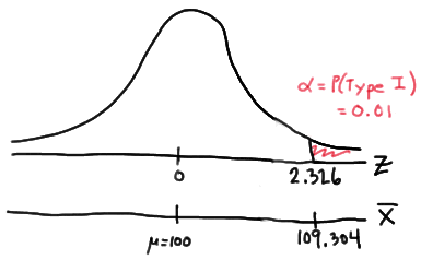
because:
\(\bar{x} = \mu + z \left( \frac{\sigma}{\sqrt{n}} \right) =100 + 2.326\left( \frac{16}{\sqrt{16}} \right)=109.304 \)
That means that the probability of rejecting the null hypothesis, when \(\mu=108\) is 0.3722 as calculated here:
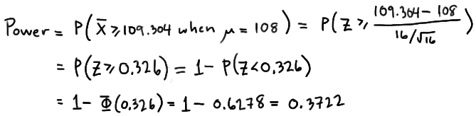
So, the power when \(\mu=108\) and \(\alpha=0.01\) is smaller (0.3722) than the power when \(\mu=108\) and \(\alpha=0.05\) (0.6406)! Perhaps we can see this graphically:
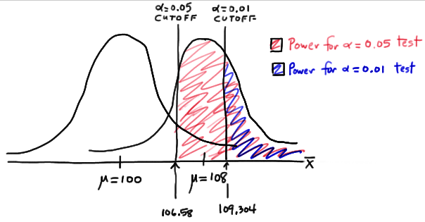
By the way, we could again alternatively look at the glass as being half-empty. In that case, the probability of a Type II error when \(\mu=108\) and \(\alpha=0.01\) is \(1-0.3722=0.6278\). In this case, the probability of a Type II error is greater than the probability of a Type II error when \(\mu=108\) and \(\alpha=0.05\).
All of this can be seen graphically by plotting the two power functions, one where \(\alpha=0.01\) and the other where \(\alpha=0.05\), simultaneously. Doing so, we get a plot that looks like this:
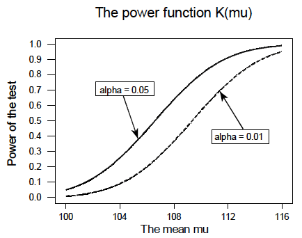
This last example illustrates that, providing the sample size \(n\) remains unchanged, a decrease in \(\alpha\) causes an increase in \(\beta\), and at least theoretically, if not practically, a decrease in \(\beta\) causes an increase in \(\alpha\). It turns out that the only way that \(\alpha\) and \(\beta\) can be decreased simultaneously is by increasing the sample size \(n\).
25.3 - Calculating Sample Size
25.3 - Calculating Sample SizeBefore we learn how to calculate the sample size that is necessary to achieve a hypothesis test with a certain power, it might behoove us to understand the effect that sample size has on power. Let's investigate by returning to our IQ example.
Example 25-3
Let \(X\) denote the IQ of a randomly selected adult American. Assume, a bit unrealistically again, that \(X\) is normally distributed with unknown mean \(\mu\) and (a strangely known) standard deviation of 16. This time, instead of taking a random sample of \(n=16\) students, let's increase the sample size to \(n=64\). And, while setting the probability of committing a Type I error to \(\alpha=0.05\), test the null hypothesis \(H_0:\mu=100\) against the alternative hypothesis that \(H_A:\mu>100\).
What is the power of the hypothesis test when \(\mu=108\), \(\mu=112\), and \(\mu=116\)?
Answer
Setting \(\alpha\), the probability of committing a Type I error, to 0.05, implies that we should reject the null hypothesis when the test statistic \(Z\ge 1.645\), or equivalently, when the observed sample mean is 103.29 or greater:
because:
\( \bar{x} = \mu + z \left(\dfrac{\sigma}{\sqrt{n}} \right) = 100 +1.645\left(\dfrac{16}{\sqrt{64}} \right) = 103.29\)
Therefore, the power function \K(\mu)\), when \(\mu>100\) is the true value, is:
\( K(\mu) = P(\bar{X} \ge 103.29 | \mu) = P \left(Z \ge \dfrac{103.29 - \mu}{16 / \sqrt{64}} \right) = 1 - \Phi \left(\dfrac{103.29 - \mu}{2} \right)\)
Therefore, the probability of rejecting the null hypothesis at the \(\alpha=0.05\) level when \(\mu=108\) is 0.9907, as calculated here:
\(K(108) = 1 - \Phi \left( \dfrac{103.29-108}{2} \right) = 1- \Phi(-2.355) = 0.9907 \)
And, the probability of rejecting the null hypothesis at the \(\alpha=0.05\) level when \(\mu=112\) is greater than 0.9999, as calculated here:
\( K(112) = 1 - \Phi \left( \dfrac{103.29-112}{2} \right) = 1- \Phi(-4.355) = 0.9999\ldots \)
And, the probability of rejecting the null hypothesis at the \(\alpha=0.05\) level when \(\mu=116\) is greater than 0.999999, as calculated here:
\( K(116) = 1 - \Phi \left( \dfrac{103.29-116}{2} \right) = 1- \Phi(-6.355) = 0.999999... \)
In summary, in the various examples throughout this lesson, we have calculated the power of testing \(H_0:\mu=100\) against \(H_A:\mu>100\) for two sample sizes ( \(n=16\) and \(n=64\)) and for three possible values of the mean ( \(\mu=108\), \(\mu=112\), and \(\mu=116\)). Here's a summary of our power calculations:
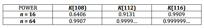
As you can see, our work suggests that for a given value of the mean \(\mu\) under the alternative hypothesis, the larger the sample size \(n\), the greater the power \(K(\mu)\). Perhaps there is no better way to see this than graphically by plotting the two power functions simultaneously, one when \(n=16\) and the other when \(n=64\):
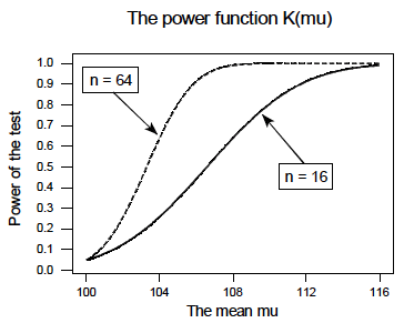
As this plot suggests, if we are interested in increasing our chance of rejecting the null hypothesis when the alternative hypothesis is true, we can do so by increasing our sample size \(n\). This benefit is perhaps even greatest for values of the mean that are close to the value of the mean assumed under the null hypothesis. Let's take a look at two examples that illustrate the kind of sample size calculation we can make to ensure our hypothesis test has sufficient power.
Example 25-4

Let \(X\) denote the crop yield of corn measured in the number of bushels per acre. Assume (unrealistically) that \(X\) is normally distributed with unknown mean \(\mu\) and standard deviation \(\sigma=6\). An agricultural researcher is working to increase the current average yield from 40 bushels per acre. Therefore, he is interested in testing, at the \(\alpha=0.05\) level, the null hypothesis \(H_0:\mu=40\) against the alternative hypothesis that \(H_A:\mu>40\). Find the sample size \(n\) that is necessary to achieve 0.90 power at the alternative \(\mu=45\).
Answer
As is always the case, we need to start by finding a threshold value \(c\), such that if the sample mean is larger than \(c\), we'll reject the null hypothesis:
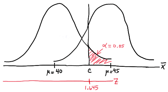
That is, in order for our hypothesis test to be conducted at the \(\alpha=0.05\) level, the following statement must hold (using our typical \(Z\) transformation):
\(c = 40 + 1.645 \left( \dfrac{6}{\sqrt{n}} \right) \) (**)
But, that's not the only condition that \(c\) must meet, because \(c\) also needs to be defined to ensure that our power is 0.90 or, alternatively, that the probability of a Type II error is 0.10. That would happen if there was a 10% chance that our test statistic fell short of \(c\) when \(\mu=45\), as the following drawing illustrates in blue:
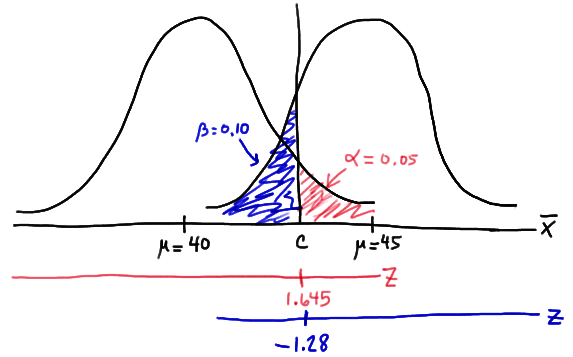
This illustration suggests that in order for our hypothesis test to have 0.90 power, the following statement must hold (using our usual \(Z\) transformation):
\(c = 45 - 1.28 \left( \dfrac{6}{\sqrt{n}} \right) \) (**)
Aha! We have two (asterisked (**)) equations and two unknowns! All we need to do is equate the equations, and solve for \(n\). Doing so, we get:
\(40+1.645\left(\frac{6}{\sqrt{n}}\right)=45-1.28\left(\frac{6}{\sqrt{n}}\right)\)
\(\Rightarrow 5=(1.645+1.28)\left(\frac{6}{\sqrt{n}}\right), \qquad \Rightarrow 5=\frac{17.55}{\sqrt{n}}, \qquad n=(3.51)^2=12.3201\approx 13\)
Now that we know we will set \(n=13\), we can solve for our threshold value c:
\( c = 40 + 1.645 \left( \dfrac{6}{\sqrt{13}} \right)=42.737 \)
So, in summary, if the agricultural researcher collects data on \(n=13\) corn plots, and rejects his null hypothesis \(H_0:\mu=40\) if the average crop yield of the 13 plots is greater than 42.737 bushels per acre, he will have a 5% chance of committing a Type I error and a 10% chance of committing a Type II error if the population mean \(\mu\) were actually 45 bushels per acre.
Example 25-5

Consider \(p\), the true proportion of voters who favor a particular political candidate. A pollster is interested in testing at the \(\alpha=0.01\) level, the null hypothesis \(H_0:9=0.5\) against the alternative hypothesis that \(H_A:p>0.5\). Find the sample size \(n\) that is necessary to achieve 0.80 power at the alternative \(p=0.55\).
Answer
In this case, because we are interested in performing a hypothesis test about a population proportion \(p\), we use the \(Z\)-statistic:
\(Z = \dfrac{\hat{p}-p_0}{\sqrt{\frac{p_0(1-p_0)}{n}}} \)
Again, we start by finding a threshold value \(c\), such that if the observed sample proportion is larger than \(c\), we'll reject the null hypothesis:
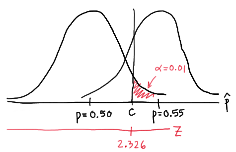
That is, in order for our hypothesis test to be conducted at the \(\alpha=0.01\) level, the following statement must hold:
\(c = 0.5 + 2.326 \sqrt{ \dfrac{(0.5)(0.5)}{n}} \) (**)
But, again, that's not the only condition that c must meet, because \(c\) also needs to be defined to ensure that our power is 0.80 or, alternatively, that the probability of a Type II error is 0.20. That would happen if there was a 20% chance that our test statistic fell short of \(c\) when \(p=0.55\), as the following drawing illustrates in blue:
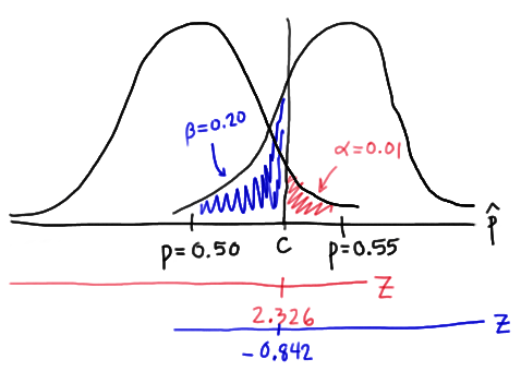
This illustration suggests that in order for our hypothesis test to have 0.80 power, the following statement must hold:
\(c = 0.55 - 0.842 \sqrt{ \dfrac{(0.55)(0.45)}{n}} \) (**)
Again, we have two (asterisked (**)) equations and two unknowns! All we need to do is equate the equations, and solve for \(n\). Doing so, we get:
\(0.5+2.326\sqrt{\dfrac{0.5(0.5)}{n}}=0.55-0.842\sqrt{\dfrac{0.55(0.45)}{n}} \\ 2.326\dfrac{\sqrt{0.25}}{\sqrt{n}}+0.842\dfrac{\sqrt{0.2475}}{\sqrt{n}}=0.55-0.5 \\ \dfrac{1}{\sqrt{n}}(1.5818897)=0.05 \qquad \Rightarrow n\approx \left(\dfrac{1.5818897}{0.05}\right)^2 = 1000.95 \approx 1001 \)
Now that we know we will set \(n=1001\), we can solve for our threshold value \(c\):
\(c = 0.5 + 2.326 \sqrt{\dfrac{(0.5)(0.5)}{1001}}= 0.5367 \)
So, in summary, if the pollster collects data on \(n=1001\) voters, and rejects his null hypothesis \(H_0:p=0.5\) if the proportion of sampled voters who favor the political candidate is greater than 0.5367, he will have a 1% chance of committing a Type I error and a 20% chance of committing a Type II error if the population proportion \(p\) were actually 0.55.
Incidentally, we can always check our work! Conducting the survey and subsequent hypothesis test as described above, the probability of committing a Type I error is:
\(\alpha= P(\hat{p} >0.5367 \text { if } p = 0.50) = P(Z > 2.3257) = 0.01 \)
and the probability of committing a Type II error is:
\(\beta = P(\hat{p} <0.5367 \text { if } p = 0.55) = P(Z < -0.846) = 0.199 \)
just as the pollster had desired.
We've illustrated several sample size calculations. Now, let's summarize the information that goes into a sample size calculation. In order to determine a sample size for a given hypothesis test, you need to specify:
-
The desired \(\alpha\) level, that is, your willingness to commit a Type I error.
-
The desired power or, equivalently, the desired \(\beta\) level, that is, your willingness to commit a Type II error.
-
A meaningful difference from the value of the parameter that is specified in the null hypothesis.
-
The standard deviation of the sample statistic or, at least, an estimate of the standard deviation (the "standard error") of the sample statistic.
Lesson 26: Best Critical Regions
Lesson 26: Best Critical RegionsIn this lesson, and the next, we focus our attention on the theoretical properties of the hypothesis tests that we've learned how to conduct for various population parameters, such as the mean \(\mu\) and the proportion p. Specifically, in this lesson, we will investigate how we know that the hypothesis tests we've learned use the best critical, that is, most powerful, regions.
26.1 - Neyman-Pearson Lemma
26.1 - Neyman-Pearson LemmaAs we learned from our work in the previous lesson, whenever we perform a hypothesis test, we should make sure that the test we are conducting has sufficient power to detect a meaningful difference from the null hypothesis. That said, how can we be sure that the T-test for a mean \(\mu\) is the "most powerful" test we could use? Is there instead a K-test or a V-test or you-name-the-letter-of-the-alphabet-test that would provide us with more power? A very important result, known as the Neyman Pearson Lemma, will reassure us that each of the tests we learned in Section 7 is the most powerful test for testing statistical hypotheses about the parameter under the assumed probability distribution. Before we can present the lemma, however, we need to:
- Define some notation
- Learn the distinction between simple and composite hypotheses
- Define what it means to have a best critical region of size \(\alpha\). First, the notation.
If \(X_1 , X_2 , \dots , X_n\) is a random sample of size n from a distribution with probability density (or mass) function \f(x; \theta)\), then the joint probability density (or mass) function of \(X_1 , X_2 , \dots , X_n\) is denoted by the likelihood function \(L (\theta)\). That is, the joint p.d.f. or p.m.f. is:
\(L(\theta) =L(\theta; x_1, x_2, ... , x_n) = f(x_1;\theta) \times f(x_2;\theta) \times ... \times f(x_n;\theta)\)
Note that for the sake of ease, we drop the reference to the sample \(X_1 , X_2 , \dots , X_n\) in using \(L (\theta)\) as the notation for the likelihood function. We'll want to keep in mind though that the likelihood \(L (\theta)\) still depends on the sample data.
Now, the definition of simple and composite hypotheses.
- Simple hypothesis
-
If a random sample is taken from a distribution with parameter \(\theta\), a hypothesis is said to be a simple hypothesis if the hypothesis uniquely specifies the distribution of the population from which the sample is taken. Any hypothesis that is not a simple hypothesis is called a composite hypothesis.
Example 26-1

Suppose \(X_1 , X_2 , \dots , X_n\) is a random sample from an exponential distribution with parameter \(\theta\). Is the hypothesis \(H \colon \theta = 3\) a simple or a composite hypothesis?
Answer
The p.d.f. of an exponential random variable is:
\(f(x) = \dfrac{1}{\theta}e^{-x/\theta} \)
for \(x ≥ 0\). Under the hypothesis \(H \colon \theta = 3\), the p.d.f. of an exponential random variable is:
\(f(x) = \dfrac{1}{3}e^{-x/3} \)
for \(x ≥ 0\). Because we can uniquely specify the p.d.f. under the hypothesis \(H \colon \theta = 3\), the hypothesis is a simple hypothesis.
Example 26-2

Suppose \(X_1 , X_2 , \dots , X_n\) is a random sample from an exponential distribution with parameter \(\theta\). Is the hypothesis \(H \colon \theta > 2\) a simple or a composite hypothesis?
Answer
Again, the p.d.f. of an exponential random variable is:
\(f(x) = \dfrac{1}{\theta}e^{-x/\theta} \)
for \(x ≥ 0\). Under the hypothesis \(H \colon \theta > 2\), the p.d.f. of an exponential random variable could be:
\(f(x) = \dfrac{1}{3}e^{-x/3} \)
for \(x ≥ 0\). Or, the p.d.f. could be:
\(f(x) = \dfrac{1}{22}e^{-x/22} \)
for \(x ≥ 0\). The p.d.f. could, in fact, be any of an infinite number of possible exponential probability density functions. Because the p.d.f. is not uniquely specified under the hypothesis \(H \colon \theta > 2\), the hypothesis is a composite hypothesis.
Example 26-3

Suppose \(X_1 , X_2 , \dots , X_n\) is a random sample from a normal distribution with mean \(\mu\) and unknown variance \(\sigma^2\). Is the hypothesis \(H \colon \mu = 12\) a simple or a composite hypothesis?
Answer
The p.d.f. of a normal random variable is:
\(f(x)= \dfrac{1}{\sigma\sqrt{2\pi}} exp \left[-\dfrac{(x-\mu)^2}{2\sigma^2} \right] \)
for \(−∞ < x < ∞, −∞ < \mu < ∞\), and \(\sigma > 0\). Under the hypothesis \(H \colon \mu = 12\), the p.d.f. of a normal random variable is:
\(f(x)= \dfrac{1}{\sigma\sqrt{2\pi}} exp \left[-\dfrac{(x-12)^2}{2\sigma^2} \right] \)
for \(−∞ < x < ∞\) and \(\sigma > 0\). In this case, the mean parameter \( \mu = 12\) is uniquely specified in the p.d.f., but the variance \(\sigma^2\) is not. Therefore, the hypothesis \(H \colon \mu = 12\) is a composite hypothesis.
And, finally, the definition of a best critical region of size \(\alpha\).
- Size of \(alpha\)
-
Consider the test of the simple null hypothesis \(H_0 \colon \theta = \theta_0\) against the simple alternative hypothesis \(H_A \colon \theta = \theta_a\). Let C and D be critical regions of size \(\alpha\), that is, let:
\(\alpha = P(C;\theta_0) \) and \(\alpha = P(D;\theta_0) \)
Then, C is a best critical region of size \(\alpha\) if the power of the test at \(\theta = \theta_a\) is the largest among all possible hypothesis tests. More formally, C is the best critical region of size \(\alpha\) if, for every other critical region D of size \(\alpha\), we have:
\(P(C;\theta_\alpha) \ge P(D;\theta_\alpha)\)
that is, C is the best critical region of size \(\alpha\) if the power of C is at least as great as the power of every other critical region D of size \(\alpha\). We say that C is the most powerful size \(\alpha\) test.
Now that we have clearly defined what we mean for a critical region C to be "best," we're ready to turn to the Neyman Pearson Lemma to learn what form a hypothesis test must take in order for it to be the best, that is, to be the most powerful test.
Suppose we have a random sample \(X_1 , X_2 , \dots , X_n\) from a probability distribution with parameter \(\theta\). Then, if C is a critical region of size \(\alpha\) and k is a constant such that:
\( \dfrac{L(\theta_0)}{L(\theta_\alpha)} \le k \) inside the critical region C
and:
\( \dfrac{L(\theta_0)}{L(\theta_\alpha)} \ge k \) outside the critical region C
then C is the best, that is, most powerful, critical region for testing the simple null hypothesis \(H_0 \colon \theta = \theta_0\) against the simple alternative hypothesis \(H_A \colon \theta = \theta_a\).
Proof
See Hogg and Tanis, pages 400-401 (8th edition pages 513-14).
Well, okay, so perhaps the proof isn't all that particularly enlightening, but perhaps if we take a look at a simple example, we'll become more enlightened. Suppose X is a single observation (that's one data point!) from a normal population with unknown mean \(\mu\) and known standard deviation \(\sigma = 1/3\). Then, we can apply the Nehman Pearson Lemma when testing the simple null hypothesis \(H_0 \colon \mu = 3\) against the simple alternative hypothesis \(H_A \colon \mu = 4\). The lemma tells us that, in order to be the most powerful test, the ratio of the likelihoods:
\(\dfrac{L(\mu_0)}{L(\mu_\alpha)} = \dfrac{L(3)}{L(4)} \)
should be small for sample points X inside the critical region C ("less than or equal to some constant k") and large for sample points X outside of the critical region ("greater than or equal to some constant k"). In this case, because we are dealing with just one observation X, the ratio of the likelihoods equals the ratio of the normal probability curves:
\( \dfrac{L(3)}{L(4)}= \dfrac{f(x; 3, 1/9)}{f(x; 4, 1/9)} \)
Then, the following drawing summarizes the situation:
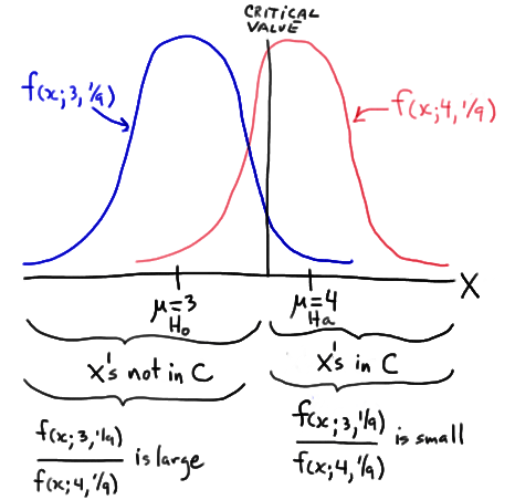
In short, it makes intuitive sense that we would want to reject \(H_0 \colon \mu = 3\) in favor of \(H_A \colon \mu = 4\) if our observed x is large, that is, if our observed x falls in the critical region C. Well, as the drawing illustrates, it is those large X values in C for which the ratio of the likelihoods is small; and, it is for the small X values not in C for which the ratio of the likelihoods is large. Just as the Neyman Pearson Lemma suggests!
Well, okay, that's the intuition behind the Neyman Pearson Lemma. Now, let's take a look at a few examples of the lemma in action.
Example 26-4
Suppose X is a single observation (again, one data point!) from a population with probabilitiy density function given by:
\(f(x) = \theta x^{\theta -1}\)
for 0 < x < 1. Find the test with the best critical region, that is, find the most powerful test, with significance level \(\alpha = 0.05\), for testing the simple null hypothesis \(H_{0} \colon \theta = 3 \) against the simple alternative hypothesis \(H_{A} \colon \theta = 2 \).
Answer
Because both the null and alternative hypotheses are simple hypotheses, we can apply the Neyman Pearson Lemma in an attempt to find the most powerful test. The lemma tells us that the ratio of the likelihoods under the null and alternative must be less than some constant k. Again, because we are dealing with just one observation X, the ratio of the likelihoods equals the ratio of the probability density functions, giving us:
\( \dfrac{L(\theta_0)}{L(\theta_\alpha)}= \dfrac{3x^{3-1}}{2x^{2-1}}= \dfrac{3}{2}x \le k \)
That is, the lemma tells us that the form of the rejection region for the most powerful test is:
\( \dfrac{3}{2}x \le k \)
or alternatively, since (2/3)k is just a new constant \(k^*\), the rejection region for the most powerful test is of the form:
\(x < \dfrac{2}{3}k = k^* \)
Now, it's just a matter of finding \(k^*\), and our work is done. We want \(\alpha\) = P(Type I Error) = P(rejecting the null hypothesis when the null hypothesis is true) to equal 0.05. In order for that to happen, the following must hold:
\(\alpha = P( X < k^* \text{ when } \theta = 3) = \int_{0}^{k^*} 3x^2dx = 0.05 \)
Doing the integration, we get:
\( \left[ x^3\right]^{x=k^*}_{x=0} = (k^*)^3 =0.05 \)
And, solving for \(k^*\), we get:
\(k^* =(0.05)^{1/3} = 0.368 \)
That is, the Neyman Pearson Lemma tells us that the rejection region of the most powerful test for testing \(H_{0} \colon \theta = 3 \) against \(H_{A} \colon \theta = 2 \), under the assumed probability distribution, is:
\(x < 0.368 \)
That is, among all of the possible tests for testing \(H_{0} \colon \theta = 3 \) against \(H_{A} \colon \theta = 2 \), based on a single observation X and with a significance level of 0.05, this test has the largest possible value for the power under the alternative hypohthesis, that is, when \(\theta = 2\).
Example 26-5

Suppose \(X_1 , X_2 , \dots , X_n\) is a random sample from a normal population with mean \(\mu\) and variance 16. Find the test with the best critical region, that is, find the most powerful test, with a sample size of \(n = 16\) and a significance level \(\alpha = 0.05\) to test the simple null hypothesis \(H_{0} \colon \mu = 10 \) against the simple alternative hypothesis \(H_{A} \colon \mu = 15 \).
Answer
Because the variance is specified, both the null and alternative hypotheses are simple hypotheses. Therefore, we can apply the Neyman Pearson Lemma in an attempt to find the most powerful test. The lemma tells us that the ratio of the likelihoods under the null and alternative must be less than some constant k:
\( \dfrac{L(10)}{L(15)}= \dfrac{(32\pi)^{-16/2} exp \left[ -(1/32)\sum_{i=1}^{16}(x_i -10)^2 \right]}{(32\pi)^{-16/2} exp \left[ -(1/32)\sum_{i=1}^{16}(x_i -15)^2 \right]} \le k \)
Simplifying, we get:
\(exp \left[ - \left( \dfrac{1}{32} \right) \left( \sum_{i=1}^{16}(x_i -10)^2 - \sum_{i=1}^{16}(x_i -15)^2 \right) \right] \le k \)
And, simplifying yet more, we get:
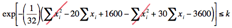
Now, taking the natural logarithm of both sides of the inequality, collecting like terms, and multiplying through by 32, we get:
\(-10\Sigma x_i +2000 \le 32ln(k)\)
And, moving the constant term on the left-side of the inequality to the right-side, and dividing through by −160, we get:
\(\dfrac{1}{16}\Sigma x_i \ge -\frac{1}{160}(32ln(k)-2000) \)
That is, the Neyman Pearson Lemma tells us that the rejection region for the most powerful test for testing \(H_{0} \colon \mu = 10 \) against \(H_{A} \colon \mu = 15 \), under the normal probability model, is of the form:
\(\bar{x} \ge k^* \)
where \(k^*\) is selected so that the size of the critical region is \(\alpha = 0.05\). That's simple enough, as it just involves a normal probabilty calculation! Under the null hypothesis, the sample mean is normally distributed with mean 10 and standard deviation 4/4 = 1. Therefore, the critical value \(k^*\) is deemed to be 11.645:
That is, the Neyman Pearson Lemma tells us that the rejection region for the most powerful test for testing \(H_{0} \colon \mu = 10 \) against \(H_{A} \colon \mu = 15 \), under the normal probability model, is:
\(\bar{x} \ge 11.645 \)
The power of such a test when \(\mu = 15\) is:
\( P(\bar{X} > 11.645 \text{ when } \mu = 15) = P \left( Z > \dfrac{11.645-15}{\sqrt{16} / \sqrt{16} } \right) = P(Z > -3.36) = 0.9996 \)
The power can't get much better than that, and the Neyman Pearson Lemma tells us that we shouldn't expect it to get better! That is, the Lemma tells us that there is no other test out there that will give us greater power for testing \(H_{0} \colon \mu = 10 \) against \(H_{A} \colon \mu = 15 \).
26.2 - Uniformly Most Powerful Tests
26.2 - Uniformly Most Powerful TestsThe Neyman Pearson Lemma is all well and good for deriving the best hypothesis tests for testing a simple null hypothesis against a simple alternative hypothesis, but the reality is that we typically are interested in testing a simple null hypothesis, such as \(H_0 \colon \mu = 10\) against a composite alternative hypothesis, such as \(H_A \colon \mu > 10\). The good news is that we can extend the Neyman Pearson Lemma to account for composite alternative hypotheses, providing we take into account each simple alternative specified in H_A. Doing so creates what is called a uniformly most powerful (or UMP) test.
- Uniformly Most Powerful (UMP) test
-
A test defined by a critical region C of size \(\alpha\) is a uniformly most powerful (UMP) test if it is a most powerful test against each simple alternative in the alternative hypothesis \(H_A\). The critical region C is called a uniformly most powerful critical region of size \(\alpha\).
Let's demonstrate by returning to the normal example from the previous page, but this time specifying a composite alternative hypothesis.
Example 26-6

Suppose \(X_1, X_2, \colon, X_n\) is a random sample from a normal population with mean \(\mu\) and variance 16. Find the test with the best critical region, that is, find the uniformly most powerful test, with a sample size of \(n = 16\) and a significance level \(\alpha\) = 0.05 to test the simple null hypothesis \(H_0: \mu = 10\) against the composite alternative hypothesis \(H_A: \mu > 10\).
Answer
For each simple alternative in \(H_A , \mu = \mu_a\), say, the ratio of the likelihood functions is:
\( \dfrac{L(10)}{L(\mu_\alpha)}= \dfrac{(32\pi)^{-16/2} exp \left[ -(1/32)\sum_{i=1}^{16}(x_i -10)^2 \right]}{(32\pi)^{-16/2} exp \left[ -(1/32)\sum_{i=1}^{16}(x_i -\mu_\alpha)^2 \right]} \le k \)
Simplifying, we get:
\(exp \left[ - \left(\dfrac{1}{32} \right) \left(\sum_{i=1}^{16}(x_i -10)^2 - \sum_{i=1}^{16}(x_i -\mu_\alpha)^2 \right) \right] \le k \)
And, simplifying yet more, we get:
Taking the natural logarithm of both sides of the inequality, collecting like terms, and multiplying through by 32, we get:
\( -2(\mu_\alpha - 10) \sum x_i +16 (\mu_{\alpha}^{2} - 10^2) \le 32 ln(k) \)
Moving the constant term on the left-side of the inequality to the right-side, and dividing through by \(-16(2(\mu_\alpha - 10)) \), we get:
\( \dfrac{1}{16} \sum x_i \ge - \dfrac{1}{16(2(\mu_\alpha - 10))}(32 ln(k) - 16(\mu_{\alpha}^{2} - 10^2)) = k^* \)
In summary, we have shown that the ratio of the likelihoods is small, that is:
\(\dfrac{L(10)}{L(\mu_\alpha)} \le k \)
if and only if:
\( \bar{x} \ge k^*\)
Therefore, the best critical region of size \(\alpha\) for testing \(H_0: \mu = 10\) against each simple alternative \(H_A \colon \mu = \mu_a\), where \(\mu_a > 10\), is given by:
\( C= \left\{ (x_1, x_1, ... , x_n): \bar{x} \ge k^* \right\} \)
where \(k^*\) is selected such that the probability of committing a Type I error is \(\alpha\), that is:
\( \alpha = P(\bar{X} \ge k^*) \text{ when } \mu = 10 \)
Because the critical region C defines a test that is most powerful against each simple alternative \(\mu_a > 10\), this is a uniformly most powerful test, and C is a uniformly most powerful critical region of size \(\alpha\).
Lesson 27: Likelihood Ratio Tests
Lesson 27: Likelihood Ratio TestsIn this lesson, we'll learn how to apply a method for developing a hypothesis test for situations in which both the null and alternative hypotheses are composite. That's not completely accurate. The method, called the likelihood ratio test, can be used even when the hypotheses are simple, but it is most commonly used when the alternative hypothesis is composite. Throughout the lesson, we'll continue to assume that we know the the functional form of the probability density (or mass) function, but we don't know the value of one (or more) of its parameters. That is, we might know that the data come from a normal distrbution, but we don't know the mean or variance of the distribution, and hence the interest in performing a hypothesis test about the unknown parameter(s).
27.1 - A Definition and Simple Example
27.1 - A Definition and Simple ExampleThe title of this page is a little risky, as there are few simple examples when it comes to likelihood ratio testing! But, we'll work to make the example as simple as possible, namely by assuming again, unrealistically, that we know the population variance, but not the population mean. Before we state the definition of a likelihood ratio test, and then investigate our simple, but unrealistic, example, we first need to define some notation that we'll use throughout the lesson.
We'll assume that the probability density (or mass) function of X is \(f(x;\theta)\) where \(\theta\) represents one or more unknown parameters. Then:
- Let \(\Omega\) (greek letter "omega") denote the total possible parameter space of \(\theta\), that is, the set of all possible values of \(\theta\) as specified in totality in the null and alternative hypotheses.
- Let \(H_0 : \theta \in \omega\) denote the null hypothesis where \(\omega\) (greek letter "omega") is a subset of the parameter space \(\Omega\).
- Let \(H_A : \theta \in \omega'\) denote the alternative hypothesis where \(\omega '\) is the complement of \(\omega\) with respect to the parameter space \(\Omega\).
Let's make sure we are clear about that phrase "where \(\omega '\) is the complement of \(\omega\) with respect to the parameter space \(\Omega\)."
Example 27-1
If the total parameter space of the mean \(\mu\) is \(\Omega = {\mu: −∞ < \mu < ∞}\) and the null hypothesis is specified as \(H_0: \mu = 3\), how should we specify the alternative hypothesis so that the alternative parameter space is the complement of the null parameter space?
Answer
If the null parameter space is \(\Omega = {\mu: \mu = 3}\), then the alternative parameter space is everything that is in \(\Omega = {\mu: −∞ < \mu < ∞}\) that is not in \(\Omega\). That is, the alternative parameter space is \(\Omega ' = {\mu: \mu ≠ 3}\). And, so the alternative hypothesis is:
\(H_A : \mu \ne 3\)
In this case, we'd be interested in deriving a two-tailed test.
Example 27-2
If the alternative hypothesis is \(H_A: \mu > 3\), how should we (technically) specify the null hypothesis so that the null parameter space is the complement of the alternative parameter space?
Answer
If the alternative parameter space is (\omega ' = {\mu: \mu > 3}\), then the null parameter space is \(\omega = {\mu: \mu ≤ 3}\). And, so the null hypothesis is:
\(H_0 : \mu \le 3\)
Now, the reality is that some authors do specify the null hypothesis as such, even when they mean \(H_0: \mu = 3\). Ours don't, and so we won't. (That's why I put that "technically" in parentheses up above.) At any rate, in this case, we'd be interested in deriving a one-tailed test.
Definition. Let:
-
\(L(\hat{\omega})\) denote the maximum of the likelihood function with respect to \(\theta\) when \(\theta\) is in the null parameter space \(\omega\).
-
\(L(\hat{\Omega})\) denote the maximum of the likelihood function with respect to \(\theta\) when \(\theta\) is in the entire parameter space \(\Omega\).
Then, the likelihood ratio is the quotient:
\(\lambda = \dfrac{L(\hat{\omega})}{L(\hat{\Omega})}\)
And, to test the null hypothesis \(H_0 : \theta \in \omega\) against the alternative hypothesis \(H_A : \theta \in \omega'\), the critical region for the likelihood ratio test is the set of sample points for which:
\(\lambda = \dfrac{L(\hat{\omega})}{L(\hat{\Omega})} \le k\)
where \(0 < k < 1\), and k is selected so that the test has a desired significance level \(\alpha\).
Example 27-3

A food processing company packages honey in small glass jars. Each jar is supposed to contain 10 fluid ounces of the sweet and gooey good stuff. Previous experience suggests that the volume X, the volume in fluid ounces of a randomly selected jar of the company's honey is normally distributed with a known variance of 2. Derive the likelihood ratio test for testing, at a significance level of \(\alpha = 0.05\), the null hypothesis \(H_0: \mu = 10\) against the alternative hypothesis H_A: \mu ≠ 10\).
Answer
Because we are interested in testing the null hypothesis \(H_0: \mu = 10\) against the alternative hypothesis \(H_A: \mu ≠ 10\) for a normal mean, our total parameter space is:
\(\Omega =\left \{\mu : -\infty < \mu < \infty \right \}\)
and our null parameter space is:
\(\omega = \left \{10\right \}\)
Now, to find the likelihood ratio, as defined above, we first need to find \(L(\hat{\omega})\). Well, when the null hypothesis \(H_0: \mu = 10\) is true, the mean \(\mu\) can take on only one value, namely, \(\mu = 10\). Therefore:
\(L(\hat{\omega}) = L(10)\)
We also need to find \(L(\hat{\Omega})\) in order to define the likelihood ratio. To find it, we must find the value of \(\mu\) that maximizes \(L(\mu)\). Well, we did that back when we studied maximum likelihood as a method of estimation. We showed that \(\hat{\mu} = \bar{x}\) is the maximum likelihood estimate of \(\mu\). Therefore:
\(L(\hat{\Omega}) = L(\bar{x})\)
Now, putting it all together to form the likelihood ratio, we get:
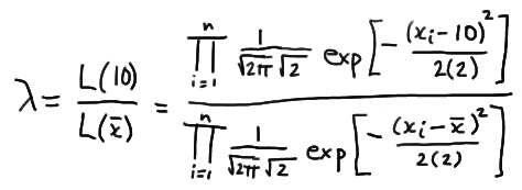
which simplifies to:
Now, let's step aside for a minute and focus just on the summation in the numerator. If we "add 0" in a special way to the quantity in parentheses:
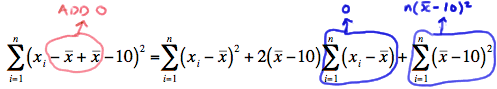
we can show that the summation can be written as:
\(\sum_{i=1}^{n}(x_i - 10)^2 = \sum_{i=1}^{n}(x_i - \bar{x})^2 + n(\bar{x} -10)^2 \)
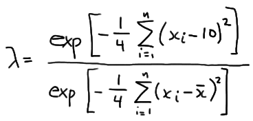
Therefore, the likelihood ratio becomes:
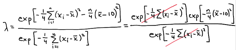
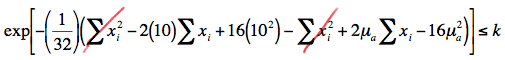
which greatly simplifies to:
\(\lambda = exp \left [-\dfrac{n}{4}(\bar{x}-10)^2 \right ]\)
Now, the likelihood ratio test tells us to reject the null hypothesis when the likelihood ratio \(\lambda\) is small, that is, when:
\(\lambda = exp\left[-\dfrac{n}{4}(\bar{x}-10)^2 \right] \le k\)
where k is chosen to ensure that, in this case, \(\alpha = 0.05\). Well, by taking the natural log of both sides of the inequality, we can show that \(\lambda ≤ k\) is equivalent to:
\( -\dfrac{n}{4}(\bar{x}-10)^2 \le \text{ln} k \)
which, by multiplying through by −4/n, is equivalent to:
\((\bar{x}-10)^2 \ge -\dfrac{4}{n} \text{ln} k \)
which is equivalent to:
\(\dfrac{|\bar{X}-10|}{\sigma / \sqrt{n}} \ge \dfrac{\sqrt{-(4/n)\text{ln} k}}{\sigma / \sqrt{n}} =k* \)
Aha! We should recognize that quantity on the left-side of the inequality! We know that:
\(Z = \dfrac{\bar{X}-10}{\sigma / \sqrt{n}} \)
follows a standard normal distribution when \(H_0: \mu = 10\). Therefore we can determine the appropriate \(k^*\) by using the standard normal table. We have shown that the likelihood ratio test tells us to reject the null hypothesis \(H_0: \mu = 10\) in favor of the alternative hypothesis \(H_A: \mu ≠ 10\) for all sample means for which the following holds:
\(\dfrac{|\bar{X}-10|}{ \sqrt{2} / \sqrt{n}} \ge z_{0.025} = 1.96 \)
Doing so will ensure that our probability of committing a Type I error is set to \(\alpha = 0.05\), as desired.
27.2 - The T-Test For One Mean
27.2 - The T-Test For One MeanWell, geez, now why would we be revisiting the t-test for a mean \(\mu\) when we have already studied it back in the hypothesis testing section? Well, the answer, it turns out, is that, as we'll soon see, the t-test for a mean \(\mu\) is the likelihood ratio test! Let's take a look!
Example 27-4

Suppose that a random sample \(X_1 , X_2 , \dots , X_n\) arises from a normal population with unknown mean \(\mu\) and unknown variance \(\sigma^2\). (Yes, back to the realistic situation, in which we don't know the population variance either.) Find the size \(\alpha\) likelihood ratio test for testing the null hypothesis \(H_0: \mu = \mu_0\) against the two-sided alternative hypothesis \(H_A: \mu ≠ \mu_0\).
Answer
Our unrestricted parameter space is:
\( \Omega = \left\{ (\mu, \sigma^2) : -\infty < \mu < \infty, 0 < \sigma^2 < \infty \right\} \)
Under the null hypothesis, the mean \(\mu\) is the only parameter that is restricted. Therefore, our parameter space under the null hypothesis is:
\( \omega = \left\{(\mu, \sigma^2) : \mu =\mu_0, 0 < \sigma^2 < \infty \right\}\)
Now, first consider the case where the mean and variance are unrestricted. We showed back when we studied maximum likelihood estimation that the maximum likelihood estimates of \(\mu\) and \(\sigma^2\) are, respectively:
\(\hat{\mu} = \bar{x} \text{ and } \hat{\sigma}^2 = \dfrac{1}{n}\sum_{i=1}^{n}(x_i - \bar{x})^2 \)
Therefore, the maximum of the likelihood function for the unrestricted parameter space is:
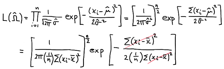
which simplifies to:
\( L(\hat{\Omega})= \left[\dfrac{ne^{-1}}{2\pi \Sigma (x_i - \bar{x})^2} \right]^{n/2} \)
Now, under the null parameter space, the maximum likelihood estimates of \(\mu\) and \(\sigma^2\) are, respectively:
\( \hat{\mu} = \mu_0 \text{ and } \hat{\sigma}^2 = \dfrac{1}{n}\sum_{i=1}^{n}(x_i - \mu_0)^2 \)
Therefore, the likelihood under the null hypothesis is:
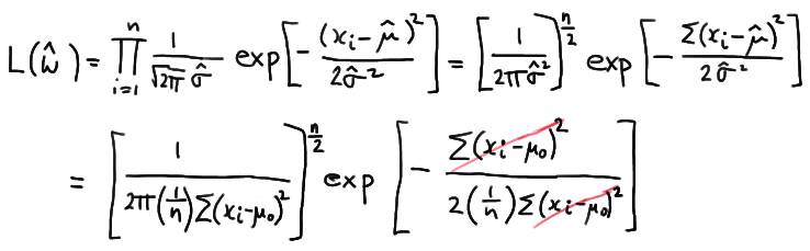
which simplifies to:
\( L(\hat{\omega})= \left[\dfrac{ne^{-1}}{2\pi \Sigma (x_i - \mu_0)^2} \right]^{n/2} \)
And now taking the ratio of the two likelihoods, we get:
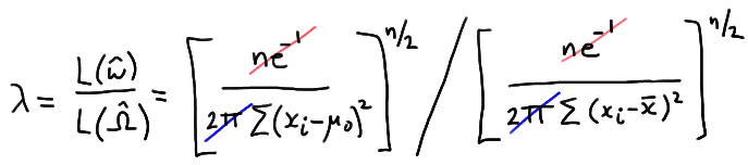
which reduces to:
\( \lambda = \left[ \dfrac{\sum_{i=1}^{n}(x_i - \bar{x})^2}{\sum_{i=1}^{n}(x_i - \mu_0)^2} \right] ^{n/2}\)
Focusing only on the denominator for a minute, let's do that trick again of "adding 0" in just the right away. Adding 0 to the quantity in the parentheses, we get:
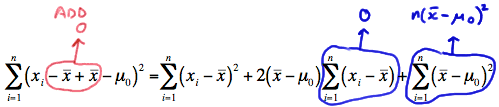
which simplifies to:
\( \sum_{i=1}^{n}(x_i - \mu_0)^2 = \sum_{i=1}^{n}(x_i - \bar{x})^2 +n(\bar{x} - \mu_0)^2 \)
Then, our likelihood ratio \(\lambda\) becomes:
\( \lambda = \left[ \dfrac{\sum_{i=1}^{n}(x_i - \bar{x})^2}{\sum_{i=1}^{n}(x_i - \mu_0)^2} \right] ^{n/2} = \left[ \dfrac{\sum_{i=1}^{n}(x_i - \bar{x})^2}{ \sum_{i=1}^{n}(x_i - \bar{x})^2 +n(\bar{x} - \mu_0)^2} \right] ^{n/2} \)
which, upon dividing through numerator and denominator by \( \sum_{i=1}^{n}(x_i - \bar{x})^2 \) simplifies to:
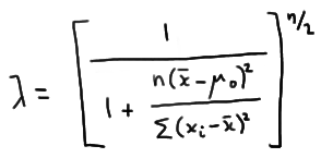
Therefore, the likelihood ratio test's critical region, which is given by the inequality \(\lambda ≤ k\), is equivalent to:
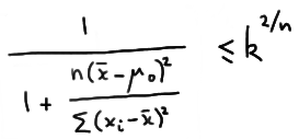
which with some minor algebraic manipulation can be shown to be equivalent to:
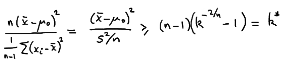
So, in a nutshell, we've shown that the likelihood ratio test tells us that for this situation we should reject the null hypothesis \(H_0: \mu= \mu_0\) in favor of the alternative hypothesis \(H_A: \mu ≠ \mu_0\) if:
\( \dfrac{(\bar{x}-\mu_0)^2 }{s^2 / n} \ge k^{*} \)
Well, okay, so I started out this page claiming that the t-test for a mean \(\mu\) is the likelihood ratio test. Is it? Well, the above critical region is equivalent to rejecting the null hypothesis if:
\( \dfrac{|\bar{x}-\mu_0| }{s / \sqrt{n}} \ge k^{**} \)
Does that look familiar? We previously learned that if \(X_1, X_2, \dots, X_n\) are normally distributed with mean \(\mu\) and variance \(\sigma^2\), then:
\( T = \dfrac{\bar{X}-\mu}{S / \sqrt{n}} \)
follows a T distribution with n − 1 degrees of freedom. So, this tells us that we should use the T distribution to choose \(k^{**}\). That is, set:
\(k^{**} = t_{\alpha /2, n-1}\)
and we have our size \(\alpha\) t-test that ensures the probability of committing a Type I error is \(\alpha\).
It turns out... we didn't know it at the time... but every hypothesis test that we derived in the hypothesis testing section is a likelihood ratio test. Back then, we derived each test using distributional results of the relevant statistic(s), but we could have alternatively, and perhaps just as easily, derived the tests using the likelihood ratio testing method.
Lesson 28: Choosing Appropriate Statistical Methods
Lesson 28: Choosing Appropriate Statistical MethodsIf we take a look back at where we've been this semester, we can quickly get the feeling as if we hiked the entire length of the 2,180 mile long Appalachian Trail. Just think about it! Among other things, we've learned about:
- Point estimation, including maximum likelihood estimation, method of moments, and sufficiency
- Confidence intervals for means, differences in two means, variances, proportions, and differences in two proportions
- Determining the sample size necessary to estimate a parameter with a certain error \(\epsilon\)
- Linear regression as a way of estimating and testing for the existence of a linear relationship between two continuous variables
- Hypothesis testing, including best critical regions and likelihood ratio tests
- Hypothesis tests for means, the equality of two means, variances, proportions and the equality of two proportions
- Determining the sample size necessary to conduct a hypothesis test for a parameter with a certain power
- One-factor analysis of variance as a way of testing for the equality of three or more population means
- Two-factor analysis of variance as a way of testing for the effect of one or more qualitative factors on a continuous variable
- Chi-square goodness-of-fit tests and contingency tables
- Using order statistics to derive distribution-free confidence intervals for percentiles
- Nonparametric methods, such as the sign test, the Wilcoxon signed rank test, the run test, and the test for randomness
- Using the Kolmogorov-Smirnov test statistic to test for the equality of a particular distribution function \(F_{0}(x)\)
- Bayesian methods
That's all well and good, but we haven't really yet had much practice with putting it altogether to choose which of the above statistical methods would be most appropriate for any given situation. For example, suppose we were interested in learning how many times each semester Penn State students go "home." What statistical method(s) would be most appropriate for answering our research question? Or, suppose we were interested in determining whether or not a higher percentage of Alaskans commit suicide than non-Alaskans. What statistical methods could we use? These are the kinds of questions we'll tackle in this lesson. The algorithm that I propose in this lesson is perhaps not flawless, but by using it, I can almost always figure out what kind of analysis is appropriate for any given situation. Choosing the correct analysis depends, at the very least, on the answer to the following four questions:
- What type of response variable do we have? More specifically, is it a continuous or categorical variable?
- How many groups are being studied or compared? Is it one, two, or more?
- What is the research question? Are we asking "is it this," so that we need to conduct a hypothesis test? Or are we asking "what is it," so that we need to calculate a point estimate or a confidence interval?
- What assumptions can we safely make about the data? Can we assume that the data are normally distributed? Can we assume the variances of two populations are equal? Are the groups dependent or independent?
As you'll soon see, upon working through the material in this lesson, choosing the correct analysis hinges on the answers to these questions. We'll first start by considering the methods that are available to us when we have one categorical (or perhaps, more specifically, binary) variable. Then, we'll move to the situation in which we have one continuous response variable. And, then two continuous measurements, before concluding with some practice questions.
28.1 - One Categorical Response
28.1 - One Categorical ResponseLet's start by considering only those methods that are appropriate for the case in which we have a binary response. You know... that means just two possible outcomes... such as, smoker or non-smoker? blue eyes or not? loves statistics or doesn't? Then, consider only those methods that are appropriate for the case in which we are studying just one group... such as, college seniors, women over the age of 60, or ash trees.
One Group with a Binary Response
Suppose we are interested in learning the extent to which the population of ash trees in the eastern United States is diseased with the emerald ash borer. Well, in that situation, we are studying just one group, namely, the population of ash trees in the eastern United States. Then, we take a random sample of n ash trees from that population and determine whether or not each tree is diseased with the emerald ash borer. In that situation, we have a binary response, namely, either the tree is or is not diseased. As soon as we determine that we are studying one group with a binary response, we should be thinking proportions, proportions, proportions. That is, a proportion is a natural way of summarizing the observed data, so therefore the statistical methods we should consider using must necessarily concern proportions. Specifically, our options are:
- performing a Z-test for one proportion
- performing a chi-square test
- calculating a Z-interval for one proportion
What we choose depends on our specific research question. If we are just interested in determining whether a majority \((p > 0.50)\) of the ash trees are diseased, a Z-test for one proportion will suffice. If we have some previous idea about the value of the proportion, \(p_0\), say of diseased trees in mind, and don't care whether the proportion is now smaller or larger than \(p_0\), then a chi-square test will suffice, as it allows for two-sided alternative hypotheses. Of course, we could just as well perform a two-sided Z-test for one proportion in that case. The P-values, and hence the final decisions, will be the same. If, on the other hand, we are only interested in estimating the unknown proportion p of diseased ash trees in the eastern United States, then we should calculate a 95% Z-interval for one proportion.
I always like to say that deciding whether to go the hypothesis test or confidence interval route depends on whether the research question involves a "is it this" or "what is it" question. That is, the research question "is the proportion of diseased trees different from 0.4?" involves conducting a hypothesis test, whereas the research question "what is the proportion of diseased trees?" involves calculating a confidence interval.
Once we've determined the appropriate statistical method, we can turn to a statistical analysis package, such as Minitab, to help with the analysis. In Minitab, we use the commands:
- Stat >> Basic Stat >> 1 Proportion... to conduct a Z-test for one proportion or to calculate a Z-interval for one proportion
- Stat >> Tables >> Cross Tabulation and Chi-Square... to conduct a chi-square test
The details about how to perform the analyses in Minitab, as well as about the assumptions that must be made, can be found in the relevant lessons.
Example 28-1

Do a majority of college students work during the semester?
Answer
The research question involves the study of one group, namely college students. The research question involves a binary response... either a student does or does not work during the semester. The research question is an "is it this?" question, and therefore involves conducting a hypothesis test. If p is the (unknown) proportion of college students who work during the semester, then we are specifically interested in testing the null hypothesis \(H_0: p = 0.50\) against the alternative hypotheses \(H_A: p > 0.50\). We can enter the resulting data into Minitab and then ask Minitab to conduct a Z-test for one proportion for us.
Incidentally, this discussion of whether or not we should conduct a hypothesis test or calculate a confidence interval is a bit like splitting hairs. That's because, as you might recall, a confidence interval can always be used to answer an "is it this?" question, too. For example, in this case, we could calculate a confidence interval for p, and then if the confidence interval only contains values greater than 0.50, then we can reject the null hypothesis \(H_0: p = 0.50\) in favor of the alternative hypotheses \(H_A: p > 0.50\). In practice, most statisticians do both, that is, conduct and report the results of both the hypothesis test and the confidence interval.
Example 28-2

What proportion of college students have an E in their last name?
Answer
The research question involves the study of one group, namely college students. The research question involves a binary response... either a student does or does not have an E in his or her last name. The research question is a "what is it?" question, and therefore involves calculating a confidence interval. If p is the (unknown) proportion of college students who have an E in their last name, then we are specifically interested in estimating p. We can enter the resulting data into Minitab and then ask Minitab to calculate a Z-interval for one proportion for us.
Two Groups with a Binary Response
Suppose we are interested in learning the extent to which the population of American men and the population of American women have a garden. In this case, we are clearly studying two groups, namely, the population of American men and the population of American women. Then, we take a random sample of \(n_1\) men and \(n_2\) women from each population and determine whether or not each person has a garden. In this case, we have a binary response, namely, either the person has a garden or does not. As soon as we determine that we are studying two groups with a binary response, we should be thinking two proportions, two proportions, two proportions. That is, a proportion is a natural way of summarizing the data observed from each population, so therefore the statistical methods we should consider using must necessarily concern two proportions. Specifically, our options are:
- performing a Z-test for two proportions
- performing a chi-square test
- calculating a Z-interval for two proportions
What we choose depends on our specific research question. Again, if the research question is an "is it this?" question, then we'd want to conduct a hypothesis test, whereas if it's a "what is it?" question, we'd want to calculate a confidence interval. For example, if we're only interested in determining whether or not the two population proportions \(p_1\) and \(p_2\) are equal, then either the Z-test for two proportions or the chi-square test would suffice. On the other hand, if we are interested in quantifying the extent to which the two proportions differ (or not), then we'd better calculate a confidence interval.
Again, once we've determined the appropriate statistical method, we can turn to a statistical analysis package, such as Minitab, to help with the analysis. In Minitab, we use the commands:
- Stat >> Basic Stat >> 2 Proportions... to conduct a Z-test for two proportions or to calculate a Z-interval for two proportions
- Stat >> Tables >> Cross Tabulation and Chi-Square... to conduct a chi-square test
The details about how to perform the analyses in Minitab, as well as about the assumptions that must be made, can be found in the relevant lessons.
Example 28-3

Do elderly males and elderly females snore at a different rate?
Answer
The research question involves the study of two groups, namely elderly males and elderly females. The research question involves a binary response... either a person does or does not snore. The research question is an "is it this?" question, and therefore involves conducting a hypothesis test. In this case, the question involves determining whether or not the difference in the two proportions \(p_1\) and \(p_2\) is 0. That is, if p1 is the (unknown) proportion of elderly males who snore, and \(p_2\) is the (unknown) proportion of elderly females who snore, then we are specifically interested in testing the null hypothesis \(H_0: p_1−p_2 = 0\) against the alternative hypotheses \(H_A: p_1−p_2 ≠ 0\). We can enter the resulting data into Minitab and then ask Minitab to conduct either a chi-square test or a Z-test for two proportions for us.
All of the examples that we have considered thus far on this page have involved a binary response variable. Let's now consider the possibility that the response is a general categorical variable.
Two or More Groups with a Categorical Response

Suppose we are interested in determining whether preference for one of four presidential candidates is independent of a voter's affiliation with a major political party (Democrat, Republican, or Independent). In this case, we are studying three groups, namely, the population of Democrat voters, the population of Republican voters, and the population of Independent voters. Then, we take a random sample of \(n_1\) Democrats, \(n_2\) Republicans, and \(n_3\) Independents, and determine whether each person prefers candidate A, B, C, or D for president. In this case, we have a general categorical response, namely, either the person prefers candidate A, B, C or D. As soon as we determine that we are studying two or more groups with a categorical response, we should be thinking chi-square test. In Minitab, we use the commands Stat >> Tables >> Cross Tabulation and Chi-Square... to conduct the test.
Example 28-4

Is the rate of smoking independent of semester standing? One-hundred randomly selected students from each of the four classes (freshmen, sophomores, juniors, and seniors) are asked about their smoking behavior (never, a few times, regularly, addicted).
Answer
The research question involves the study of four groups, namely freshmen, sophomores, juniors, and seniors. The research question involves a categorical response... either a person classifies him- or herself as having never smoked, as having smoked a few times, as a regular smoker, or as being completely addicted. The research question involves assessing the independence of the two variables, smoking and semester standing. In summarizing the data, we determine the proportion of freshmen falling into each category of smokers, the proportion of sophomores falling into each category of smokers, the proportion of juniors falling into each category of smokers, and the proportion of seniors falling into each category of smokers. We can enter the resulting data into Minitab and then ask Minitab to conduct a chi-square test for us.
28.2 - One Continuous Response
28.2 - One Continuous ResponseNow, let's turn our attention towards those methods that are appropriate for the case in which we have a continuous response. You know... that means a response that falls in an interval of values... such as, weight (in pounds), temperature (in degrees Fahreneit), or grade on a statistics final exam. First, let's consider only those methods that are appropriate for the case in which we are studying just one group... such as, high school freshmen, six-year-old girls, or moray eels.
One Group with a Continuous Response

Suppose we are interested in learning about the length of the population of moray eels. In that case, we are studying just one group, namely, the population of moray eels. Then, we take a random sample of n moray eels from that population and determine the length of each specimen selected. In that situation, we have a continuous response, namely, the length of the eel. As soon as we determine that we are studying one group with a continuous response, we should be thinking means, means, means, or .... errr.... medians, medians, medians. Which is the more appropriate summary statistic, of course, depends on the distribution of the data, that is, whether it is symmetric or skewed. At any rate, the mean or the median is a natural way of summarizing the observed data, so therefore the statistical methods we should potentially use must necessarily concern either means of medians. Specifically, our options are:
- performing a t-test for one mean
- performing a sign test or signed rank test for one median
- calculating a t-interval for one mean
- calculating a distribution-free confidence interval for a median or a general percentile
Again, what we choose depends on our specific research question. If the research question is an "is it this?" question, then we'd want to conduct a hypothesis test, whereas if it's a "what is it?" question, we'd want to calculate a confidence interval. Once we determine the appropriate statistical method, Minitab can do the dirty work for us using these commands:
- Stat >> Basic Stat >> 1-Sample t... to conduct a t-test for one mean or to calculate a t-interval for one mean
- Stat >> Nonparametrics >> 1-Sample Sign... to conduct a sign test
- Stat >> Nonparametrics >> 1-Sample Wilcoxon... to conduct a signed rank test for one median or to calculate a distribution-free confidence interval for a median
The details about how to perform the analyses in Minitab, as well as about the assumptions that must be made in each case, can be found in the relevant lessons.
Example 28-5

What is the mean length of the pointer finger of the population of college students?
Answer
The research question involves the study of one group, namely college students. The research question involves a continuous response... the length of the pointer finger of a randomly selected college student. The research question is a "what is it?" question, and therefore involves calculating a confidence interval. If \(\mu\) is the (unknown) mean length of the pointer finger of college students, then we are specifically interested in estimating \(\mu\). We can enter the resulting data into Minitab and then ask Minitab to calculate a t-interval for one mean for us.
Example 28-6

Is the mean IQ, as measured by the Stanford-Binet IQ test, of the population of graduating college seniors greater than 115?
Answer
The research question involves the study of one group, namely graduating college seniors. The research question involves a continuous response... the score on the Stanford-Binet IQ test. The research question is a "is it this?" question, and therefore involves conducting a hypothesis test. If \(\mu\) is the (unknown) mean IQ score of graduating college seniors, then we are specifically interested in testing the null hypothesis \(H_0: \mu = 115\) against the alternative hypothesis \(H_A: \mu > 115\). We can enter the resulting data into Minitab and then ask Minitab to conduct a t-test for one mean for us.
Example 28-7

Is the median annual income of American households greater than \$40,000?
Answer
The research question involves the study of one group, namely American households. The research question involves a continuous response... annual income (in dollars). The research question is a "is it this?" question, and therefore involves conducting a hypothesis test. At this point, because the response is continuous we could conduct a hypothesis test about the mean or the median. However, because it is well known that the distribution of American incomes is highly skewed, the median is a better measure of the "center" of the income distribution. Therefore, our analysis should probably concern the median. That said, if m is the (unknown) median annual income of American households, then we are specifically interested in testing the null hypothesis \(H_0: m = 40,000\) against the alternative hypothesis \(H_A: m > 40,000\). We can enter the resulting data into Minitab and then ask Minitab to conduct either a sign test or a signed rank test for one median for us.
Two Paired Groups with a Continuous Response

Suppose we are interested in comparing the heights of first-born and second-born twins. Then, we have two groups, namely that of the first-born twins and that of the second-born twins. The groups have a special characteristic, however, in that they are not independent. As you know, we say they are paired. Therefore, any analysis we perform would have to take this dependence into account. The response, height, is of course, continuous. Therefore, our analysis involves two paired groups with a continuous response, and hence our options are:
- performing a paired t-test for a mean difference
- performing a sign test or signed rank test for a median difference
- calculating a paired t-interval for a mean difference
- calculating a distribution-free confidence interval for a median (or general percentile) difference
Again, what we choose depends on our specific research question. If the research question is an "is it this?" question, then we'd want to conduct a hypothesis test, whereas if it's a "what is it?" question, we'd want to calculate a confidence interval. Once we determine the appropriate statistical method, Minitab can do the dirty work for us using these commands:
- Stat >> Basic Stat >> Paired t... to conduct a paired t-test for a mean difference or to calculate a paired t-interval for a mean difference
- Stat >> Nonparametrics >> 1-Sample Sign... to conduct a sign test for a median difference
- Stat >> Nonparametrics >> 1-Sample Wilcoxon... to conduct a signed rank test for a median difference or to calculate a distribution-free confidence interval for a median difference
The details about how to perform the analyses in Minitab, as well as about the assumptions that must be made in each case, can be found in the relevant lessons.
Example 28-8

Do people's pulse rates increase after exercise?
Answer
The research question involves the study of one group, namely people. Oops, actually if you think about it, the question involves the study of two groups, people, before exercise and people after exercise. Although the research question doesn't specifically suggest this, we should all know by now that it would be a good idea to collect the data in a paired way, that is, to measure the same people before and after exercise. Doing otherwise would introduce needless variability into the data. By measuring the same people twice, of course, removes the independence of the groups, and hence we should be thinking paired, paired, paired.
Because the research question involves a continuous response... the pulse rate, we should be thinking mean, mean, mean or median, median, median. So, we have a paired, paired, paired, mean, mean, mean or a paired, paired, paired, median, median, median. (I've been clearly writing too long today.) At any rate, the research question is clearly a "is it this?" question. It is? Clearly? Well, if \(\mu_D = \mu_{After} − \mu_{Before}\), is the (unknown) mean difference in the pulse rates, then we are specifically interested in testing the null hypothesis \(H_0: \mu_D = 0\) against the alternative hypothesis \(H_A: \mu_D > 0\). We can enter the resulting data into Minitab and then ask Minitab to conduct either a paired t-test for one mean or, alternatively, a sign test or signed-rank test for the median difference. Of course, if we went a step further, we could also ask Minitab to calculate a confidence interval for us, so that we can quantify how different the pulse rates are before and after exercise.
Two Independent Groups with a Continuous Response

Suppose we are interested in comparing the gas mileage of two different vehicles, Toyota Camry and Volkswagen Passat, say. In this case, we have two independent groups, namely that of Toyota Camry vehicles and that of Volkswagen Passat vehicles. The response, gas mileage, is a continuous measurement. Therefore, our analysis would involve two independent groups with a continuous response, and hence our options are:
- performing a two-sample t-test for the difference in two means
- performing a two-sample Wilcoxon test for a difference in two medians
- calculating a two-sample t-interval for the difference in two means
Again, what we choose depends on our specific research question. If the research question is an "is it this?" question, then we'd want to conduct a hypothesis test, whereas if it's a "what is it?" question, we'd want to calculate a confidence interval. Once we determine the appropriate statistical method, Minitab can do the dirty work for us using these commands:
- Stat >> Basic Stat >> 2-Sample t... to conduct a t-test for the difference in two means or to calculate a t-interval for the difference in two means
- Stat >> Nonparametrics >> Mann-Whitney... to conduct a variation of the two-sample Wilcoxon test for a difference in two medians
The details about how to perform the analyses in Minitab, as well as about the assumptions that must be made in each case, can be found in the relevant lessons.
Example 28-9

Do the resting pulse rates of adult males and females differ?
Answer
The research question involves the study of two independent groups, namely that of adult males and females. The research question involves a continuous response... resting pulse rates. The research question is a "is it this?" question, and therefore involves conducting a hypothesis test. If \(\mu_M\) is the (unknown) mean pulse rate of adult males, and \(\mu_F\) is the (unknown) mean pulse rate of adult females, then we are specifically interested in testing the null hypothesis:
\(H_0: \mu_M − \mu_F = 0\)
against the alternative hypothesis:
\(H_A: \mu_M − \mu_F ≠ 0\)
We can enter the resulting data into Minitab and then ask Minitab to conduct a two-sample t-test for one mean for us. Of course, we should check, as always, for the normality of the data and the equality of the population variances.
More than Two Independent Groups with a Continuous Response??

Suppose we are interested in comparing the average 5-kilometer race times of four different age groups. Because we have four independent groups and one continuous response, namely the race times, we would want to conduct a one-factor analysis of variance. If we were interested in testing whether a second factor, such as gender, had an effect on race times, then we would want to conduct a two-factor analysis of variance. We'd, of course, have to check the necessary assumptions, but once we did that, we could let Minitab do the analysis for us using these commands:
- Stat >> ANOVA >> One-way... to conduct a one-factor analysis of variance with the grouping variable in one column and the response in a second column
- Stat >> ANOVA >> One-way (Unstacked)... to conduct a one-factor analysis of variance with each group's responses being recorded in a different column
- Stat >> ANOVA >> Two-way... to conduct a two-factor analysis of variance
The details about how to perform the analyses in Minitab, as well as about the assumptions that must be made in each case, can be found in the relevant lessons.
28.3 - Two Continuous Measurements
28.3 - Two Continuous MeasurementsOne Group with Two Continuous Measurements
If we have two continuous measurements, we could consider either of two possible analyses, namely:
- Correlation
- Linear regression
Correlation helps to answer the research question "does a linear relationship exist between two continuous random variables?" Linear regression, on the other hand, helps to answer the research question "what is the linear relationship between a fixed predictor and a random variable?" In Minitab, we use the following commands:
- Stat >> Basic Statistics >> Correlation... to conduct a correlation analysis
- Stat >> Regression >> Regression... to conduct a linear regression analysis
Example 28-10

Does a (linear) relationship exist between a husband's and wife's height?
Answer
Because we are only interested in learning whether a linear relationship exists between husbands' and wives' heights, and not the nature of the relationship, we would want to conduct a correlation analysis. We can use Minitab's Stat >> Basic Statistics >> Correlation... command to test the null hypothesis:
\(H_0 : \rho = 0\)
against the alternative hypothesis:
\(H_A : \rho \ne 0\)
Example 28-11

If a randomly selected college student goes out to party ten times each month, what kind of grade point average (GPA) can he or she expect?
Answer
If x denotes the number of times a randomly selected college student goes out to party in one month, and y = the student's grade point average, then we'd be interested in estimating the slope and intercept parameters in the linear regression equation:
\(\mu_y=\alpha + \beta x\)
Of course, that's assuming that the relationship is indeed a linear relationship, but that could be verified when doing the analysis. We could use Minitab's Stat >> Regression >> Regression... command to help complete the analysis.
28.4 - Practice
28.4 - PracticeWe've pretty much reviewed now all of the analysis methods we've learned in this course, as well as when it would be appropriate to use each analysis method. In summary:
- First, ask what type of response has been measured. Do we summarize it by a proportion or a mean (median)?
- Then, ask how many groups are being studied and/or compared.
- Then, decide whether we should conduct a hypothesis test or calculate an interval estimate.
- And, of course, always check that the method's assumptions and/or conditions are met.
Try it!
For each of the following research questions, identify at least one analysis that would be appropriate for the situation.
-
Do seniors earn higher semester grade point averages than freshmen?
Answer
We have two groups, seniors and freshmen. The response is continuous. We are only interested in determining whether or not a difference between the two groups exists. Therefore, conduct a two-sample t-test for testing the difference in the mean GPA for seniors and the mean GPA for freshmen.
-
What is the relationship between the amount of alcohol consumed (in ounces) and the level of coordination (on a scale from 1 to 10)?
Answer
We have two continuous measurements, for which we are interested in quantifying the nature of the relationship. Therefore, conduct a linear regression analysis so that we can estimate:
\(\mu_y=\alpha + \beta x\)
where x denotes the amount of alcohol consumed and the level of coordination is the response y.
-
Are SAT scores and grade point averages linearly related?
Answer
We have two continuous measurements, for which we are interested in determining whether or not a linear relationship exists. Therefore, conduct a correlation analysis to test the null hypothesis:
\(H_0 : \rho = 0\)
against the alternative hypothesis:
\(H_A : \rho \ne 0\)
-
Is there a difference in the percentage of NCAA basketball players who graduate and NCAA football players who graduate?
Answer
The response is binary (graduate or not), and there are two groups being compared (NCAA basketball players and NCAA football players). Therefore, conduct a Z-test for comparing two proportions.
-
How many hours per week do PSU students study outside of class?
Answer
We have a continuous response variable (number of hours per week studied) and one group (PSU students). Therefore, calculate a one-sample t-interval for the mean \(\mu\).
-
How much more prevalent is lupus in women than in men?
Answer
We have a binary response (lupus or not), and two groups (men and women). Therefore, calculate a Z-interval for the difference in the two proportions.
-
Do PSU students drink, on average, more than one cup of coffee per day during finals week? (During finals week, a sample of students will record how many cups of coffee they drink each day.)
Answer
We have a continuous response variable (number of cups of coffee consumed per day during finals week) and one group (PSU students). Therefore, conduct a one-sample t-test for testing \(H_0: \mu = 1\) against \(H_A: \mu > 1\).
-
Is the recovery time from a migraine headache related to the treatment (A, B, C)?
Answer
We have a continuous response variable (recovery time) and three groups (A, B, C). Therefore, conduct a one-factor analysis of variance for testing \(H_0: \mu_A = \mu_B = \mu_C\) against \(H_A:\) not all \(\mu_i\) are equal.
-
Is there a relationship between political affilition (Democrat, Republican, Independent) and income level (Poor, Middle Class, Wealthy)?
Answer
We have two categorical variables for which we are interested in determining whether or not a relationship exists. Therefore, conduct a chi-square test.
-
How much heavier (in pounds) are 15-year-old boys than 13-year-old boys?
Answer
We have a continuous response (weight in pounds) and two independent groups (13-year-old and 15-year-old boys). Therefore, calculate a two-sample t-interval for the difference in the two means.
-
A random sample of 64 students were asked "do you study regularly at Pattee Library?"
Answer
We have a binary response (yes or no) and one group (students). Therefore, calculate a confidence interval for the proportion of students who study regularly at Pattee.
-
Do Goodyear tires have better tread wear than Firestone tires? Tread wear is measured in millimeters of tread remaining after 30,000 miles. Thirty cars are selected for an experiment. On each car, one Goodyear tire and one Firestone tire is placed randomly in one of two front positions.
Answer
We have a continuous response (tread wear) and two paired groups (Firestone and Goodyear tires). Therefore, conduct a paired t-test for testing whether the mean difference is 0.