8.1 - A Confidence Interval for the Mean of Y
8.1 - A Confidence Interval for the Mean of YWe have gotten so good with deriving confidence intervals for various parameters, let's just jump right in and state (and prove) the result.
Theorem
A \((1-\alpha)100\%\) confidence interval for the mean \(\mu_Y\) is:
\(\hat{y} \pm t_{\alpha/2,n-2}\sqrt{MSE} \sqrt{\dfrac{1}{n}+\dfrac{(x-\bar{x})^2}{\sum(x_i-\bar{x})^2}}\)
Proof
We know from our work in the previous lesson that a point estimate of the mean \(\mu_Y\) is:
\(\hat{y}=\hat{\alpha}+\hat{\beta}(x-\bar{x})\)
Now, recall that:
\(\hat{\alpha} \sim N\left(\alpha,\dfrac{\sigma^2}{n}\right)\) and \(\hat{\beta}\sim N\left(\beta,\dfrac{\sigma^2}{\sum_{i=1}^n (x_i-\bar{x})^2}\right)\) and \(\dfrac{n\hat{\sigma}^2}{\sigma^2}\sim \chi^2_{(n-2)}\)
are independent. Therefore, \(\hat{Y}\) is a linear combination of independent normal random variables with mean:
\(E(\hat{y})=E[\hat{\alpha}+\hat{\beta}(x-\bar{x})]=E(\hat{\alpha})+(x-\bar{x})E(\hat{\beta})=\alpha+\beta(x-\bar{x})=\mu_Y\)
and variance:
\(Var(\hat{y})=Var[\hat{\alpha}+\hat{\beta}(x-\bar{x})]=Var(\hat{\alpha})+(x-\bar{x})^2 Var(\hat{\beta})=\dfrac{\sigma^2}{n}+\dfrac{(x-\bar{x})^2\sigma^2}{\sum(x_i-\bar{x})^2}=\sigma^2\left[\dfrac{1}{n}+\dfrac{(x-\bar{x})^2}{\sum(x_i-\bar{x})^2}\right]\)
The first equality holds by the definition of \(\hat{Y}\). The second equality holds because \(\hat{\alpha}\) and \(\hat{\beta}\) are independent. The third equality comes from the distributions of \(\hat{\alpha}\) and \(\hat{\beta}\) that are recalled above. And, the last equality comes from simple algebra. Putting it all together, we have:
\(\hat{Y} \sim N\left(\mu_Y, \sigma^2\left[\dfrac{1}{n}+\dfrac{(x-\bar{x})^2}{\sum(x_i-\bar{x})^2}\right]\right)\)
Now, the definition of a \(T\) random variable tells us that:
\(T=\dfrac{\dfrac{\hat{Y}-\mu_Y}{\sigma \sqrt{\dfrac{1}{n}+\dfrac{(x-\bar{x})^2}{\sum(x_i-\bar{x})^2}}}}{\sqrt{\dfrac{n\hat{\sigma}^2}{\sigma^2}/(n-2)}}=\dfrac{\hat{Y}-\mu_Y}{\sqrt{MSE} \sqrt{\dfrac{1}{n}+\dfrac{(x-\bar{x})^2}{\sum(x_i-\bar{x})^2}}} \sim t_{n-2}\)
So, finding the confidence interval for \(\mu_Y\) again reduces to manipulating the quantity inside the parentheses of a probability statement:
\(P\left(-t_{\alpha/2,n-2} \leq \dfrac{\hat{Y}-\mu_Y}{\sqrt{MSE} \sqrt{\dfrac{1}{n}+\dfrac{(x-\bar{x})^2}{\sum(x_i-\bar{x})^2}}} \leq +t_{\alpha/2,n-2}\right)=1-\alpha\)
Upon doing the manipulation, we get that a \((1-\alpha)100\%\) confidence interval for \(\mu_Y\) is:
\(\hat{y} \pm t_{\alpha/2,n-2}\sqrt{MSE} \sqrt{\dfrac{1}{n}+\dfrac{(x-\bar{x})^2}{\sum(x_i-\bar{x})^2}}\)
as was to be proved.
Example 8-1
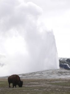
The eruptions of Old Faithful Geyser in Yellowstone National Park, Wyoming are quite regular (and hence its name). Rangers post the predicted time until the next eruption (\(y\), in minutes) based on the duration of the previous eruption (\(x\), in minutes). Using the data collected on 107 eruptions from a park geologist, R. A. Hutchinson, what is the mean time until the next eruption if the previous eruption lasted 4.8 minutes? lasted 3.5 minutes? (Photo credit: Tony Lehrman)
Answer
The easiest (and most practical!) way of calculating the confidence interval for the mean is to let Minitab do the work for us. Here's what the resulting analysis looks like:
The regression equation is NEXT = 33.828 + 10.741 DURATION
Analysis of Variance
| Source | DF | SS | MS | F | P |
|---|---|---|---|---|---|
| Regression | 1 | 13133 | 13133 | 294.08 | 0.000 |
| Residual Error | 105 | 4689 | 45 | 0.000 | |
|
Total |
106 | 17822 |
|
| New Obs |
Fit | SE Fit | 95% CI | 95% PI |
|---|---|---|---|---|
| 4.8 | 85.385 | 1.059 | (83.286, 87.484) | (71.969, 98.801) |
| 3.5 | 77.422 | 0.646 | (70.140, 72.703) | (58.109, 84.734) |
That is, we can be 95% confident that, if the previous eruption lasted 4.8 minutes, then the mean time until the next eruption is between 83.286 and 87.484 minutes. And, we can be 95% confident that, if the previous eruption lasted 3.5 minutes, then the mean time until the next eruption is between 70.140 and 72.703 minutes.
Let's do one of the calculations by hand, though. When the previous eruption lasted \(x=4.8\) minutes, then the predicted time until the next eruption is:
\(\hat{y}=33.828 + 10.741(4.8)=85.385\)
Now, we can use Minitab or a probability calculator to determine that \(t_{0.025, 105}=1.9828\). We can also use Minitab to determine that MSE equals 44.6 (it is rounded to 45 in the above output), the mean duration is 3.46075 minutes, and:
\(\sum\limits_{i=1}^n (x_i-\bar{x})^2=113.835\)
Putting it all together, we get:
\(85.385 \pm 1.9828 \sqrt{44.66} \sqrt{\dfrac{1}{107}+\dfrac{(4.8-3.46075)^2}{113.835}}\)
which simplifies to this:
\(85.385 \pm 2.099\)
and finally this:
\((83.286,87.484)\)
as we (thankfully) obtained previously using Minitab. Incidentally, you might note that the length of the confidence interval for \(\mu_Y\) when \(x=4.8\) is:
\(87.484-83.286=4.198\)
and the length of the confidence interval when \(x=3.5\) is:
\(72.703-70.140=2.563\)
Hmmm. That suggests that the confidence interval is narrower when the \(x\) value is close to the mean of all of the \(x\) values. That is, in fact, one generalization, among others, that we can make about the length of the confidence interval for \(\mu_Y\).
Ways of Getting a Narrow(er) Confidence Interval for \(\mu_Y\)
If we take a look at the formula for the confidence interval for \(\mu_Y\):
\(\hat{y} \pm t_{\alpha/2,n-2}\sqrt{MSE} \sqrt{\dfrac{1}{n}+\dfrac{(x-\bar{x})^2}{\sum(x_i-\bar{x})^2}}\)
we can determine four ways in which we can get a narrow confidence interval for \(\mu_Y\). We can:
-
Estimate the mean \(\mu_Y\) at the mean of the predictor values. That's because when \(x=\bar{x}\), the term circled in blue:
\(\hat{y} \pm t_{\alpha / 2, n-2} \sqrt{M S E} \sqrt{\frac{1}{n}+\frac{\color{blue}\boxed{\color{black}(x-\bar{x})^{2}}}{\sum\left(x_{i}-\bar{x}\right)^{2}}}\)
-
contributes nothing to the length of the interval. That is, the shortest confidence interval for \(\mu_Y\) occurs when \(x=\bar{x}\).
-
Decrease the confidence level. That's because, the smaller the confidence level, the smaller the term circled in blue:
\(\hat{y} \pm \color{blue}\boxed{\color{black}t_{\alpha / 2, n-2}}\color{black} \sqrt{M S E} \sqrt{\frac{1}{n}+\frac{(x-\bar{x})^{2}}{\sum\left(x_{i}-\bar{x}\right)^{2}}}\)
-
Increase the sample size. That's because, the larger the sample size, the larger the term circled in blue:
\(\hat{y} \pm t_{\alpha / 2, n-2} \sqrt{M S E} \sqrt{\frac{1}{\color{blue}\boxed{\color{black}n}}+\frac{(x-\bar{x})^{2}}{\sum\left(x_{i}-\bar{x}\right)^{2}}}\)
and therefore the shorter the length of the interval.
-
Choose predictor values \(x_i\) so that they are quite spread out. That's because the more spread out the predictor values, the larger the term circled in blue:
\(\hat{y} \pm t_{\alpha / 2, n-2} \sqrt{M S E} \sqrt{\frac{1}{n}+\frac{(x-\bar{x})^{2}}{\color{blue}\boxed{\color{black}\sum\left(x_{i}-\bar{x}\right)^{2}}}}\)
and therefore the shorter the length of the interval.