25.2 - Power Functions
25.2 - Power FunctionsExample 25-2

Let's take a look at another example that involves calculating the power of a hypothesis test.
Let \(X\) denote the IQ of a randomly selected adult American. Assume, a bit unrealistically, that \(X\) is normally distributed with unknown mean \(\mu\) and standard deviation 16. Take a random sample of \(n=16\) students, so that, after setting the probability of committing a Type I error at \(\alpha=0.05\), we can test the null hypothesis \(H_0:\mu=100\) against the alternative hypothesis that \(H_A:\mu>100\).
What is the power of the hypothesis test if the true population mean were \(\mu=108\)?
Answer
Setting \(\alpha\), the probability of committing a Type I error, to 0.05, implies that we should reject the null hypothesis when the test statistic \(Z\ge 1.645\), or equivalently, when the observed sample mean is 106.58 or greater:
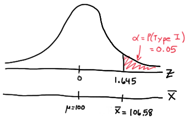
because we transform the test statistic \(Z\) to the sample mean by way of:
\(Z=\dfrac{\bar{X}-\mu}{\frac{\sigma}{\sqrt{n}}}\qquad \Rightarrow \bar{X}=\mu+Z\dfrac{\sigma}{\sqrt{n}} \qquad \bar{X}=100+1.645\left(\dfrac{16}{\sqrt{16}}\right)=106.58\)
Now, that implies that the power, that is, the probability of rejecting the null hypothesis, when \(\mu=108\) is 0.6406 as calculated here (recalling that \(Phi(z)\) is standard notation for the cumulative distribution function of the standard normal random variable):
\( \text{Power}=P(\bar{X}\ge 106.58\text{ when } \mu=108) = P\left(Z\ge \dfrac{106.58-108}{\frac{16}{\sqrt{16}}}\right) \\ = P(Z\ge -0.36)=1-P(Z<-0.36)=1-\Phi(-0.36)=1-0.3594=0.6406 \)
and illustrated here:
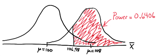
In summary, we have determined that we have (only) a 64.06% chance of rejecting the null hypothesis \(H_0:\mu=100\) in favor of the alternative hypothesis \(H_A:\mu>100\) if the true unknown population mean is in reality \(\mu=108\).
What is the power of the hypothesis test if the true population mean were \(\mu=112\)?
Answer
Because we are setting \(\alpha\), the probability of committing a Type I error, to 0.05, we again reject the null hypothesis when the test statistic \(Z\ge 1.645\), or equivalently, when the observed sample mean is 106.58 or greater. That means that the probability of rejecting the null hypothesis, when \(\mu=112\) is 0.9131 as calculated here:
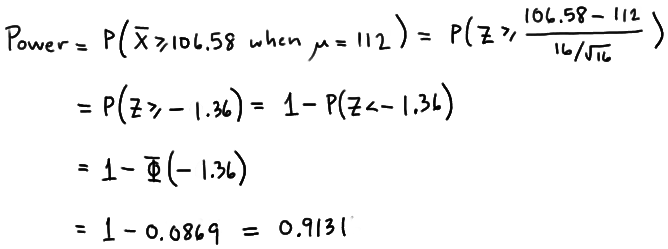
\( \text{Power}=P(\bar{X}\ge 106.58\text{ when }\mu=112)=P\left(Z\ge \frac{106.58-112}{\frac{16}{\sqrt{16}}}\right) \\ = P(Z\ge -1.36)=1-P(Z<-1.36)=1-\Phi(-1.36)=1-0.0869=0.9131 \)
and illustrated here:
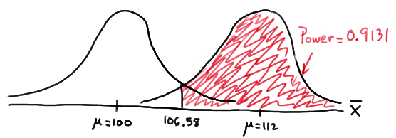
In summary, we have determined that we now have a 91.31% chance of rejecting the null hypothesis \(H_0:\mu=100\) in favor of the alternative hypothesis \(H_A:\mu>100\) if the true unknown population mean is in reality \(\mu=112\). Hmm.... it should make sense that the probability of rejecting the null hypothesis is larger for values of the mean, such as 112, that are far away from the assumed mean under the null hypothesis.
What is the power of the hypothesis test if the true population mean were \(\mu=116\)?
Answer
Again, because we are setting \(\alpha\), the probability of committing a Type I error, to 0.05, we reject the null hypothesis when the test statistic \(Z\ge 1.645\), or equivalently, when the observed sample mean is 106.58 or greater. That means that the probability of rejecting the null hypothesis, when \(\mu=116\) is 0.9909 as calculated here:

\(\text{Power}=P(\bar{X}\ge 106.58\text{ when }\mu=116) =P\left(Z\ge \dfrac{106.58-116}{\frac{16}{\sqrt{16}}}\right) = P(Z\ge -2.36)=1-P(Z<-2.36)= 1-\Phi(-2.36)=1-0.0091=0.9909 \)
and illustrated here:

In summary, we have determined that, in this case, we have a 99.09% chance of rejecting the null hypothesis \(H_0:\mu=100\) in favor of the alternative hypothesis \(H_A:\mu>100\) if the true unknown population mean is in reality \(\mu=116\). The probability of rejecting the null hypothesis is the largest yet of those we calculated, because the mean, 116, is the farthest away from the assumed mean under the null hypothesis.
Are you growing weary of this? Let's summarize a few things we've learned from engaging in this exercise:
- First and foremost, my instructor can be tedious at times..... errrr, I mean, first and foremost, the power of a hypothesis test depends on the value of the parameter being investigated. In the above, example, the power of the hypothesis test depends on the value of the mean \(\mu\).
- As the actual mean \(\mu\) moves further away from the value of the mean \(\mu=100\) under the null hypothesis, the power of the hypothesis test increases.
It's that first point that leads us to what is called the power function of the hypothesis test. If you go back and take a look, you'll see that in each case our calculation of the power involved a step that looks like this:
\(\text{Power } =1 - \Phi (z) \) where \(z = \frac{106.58 - \mu}{16 / \sqrt{16}} \)
That is, if we use the standard notation \(K(\mu)\) to denote the power function, as it depends on \(\mu\), we have:
\(K(\mu) = 1- \Phi \left( \frac{106.58 - \mu}{16 / \sqrt{16}} \right) \)
So, the reality is your instructor could have been a whole lot more tedious by calculating the power for every possible value of \(\mu\) under the alternative hypothesis! What we can do instead is create a plot of the power function, with the mean \(\mu\) on the horizontal axis and the power \(K(\mu)\) on the vertical axis. Doing so, we get a plot in this case that looks like this:
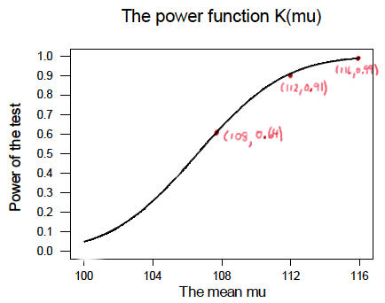
Now, what can we learn from this plot? Well:
-
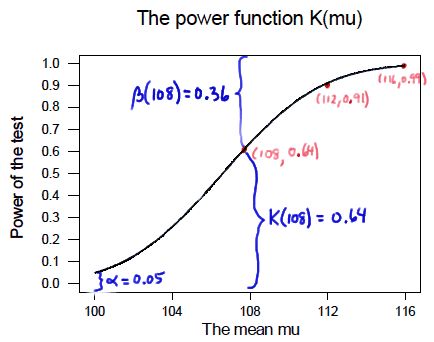
We can see that \(\alpha\) (the probability of a Type I error), \(\beta\) (the probability of a Type II error), and \(K(\mu)\) are all represented on a power function plot, as illustrated here:
-
We can see that the probability of a Type I error is \(\alpha=K(100)=0.05\), that is, the probability of rejecting the null hypothesis when the null hypothesis is true is 0.05.
-
We can see the power of a test \(K(\mu)\), as well as the probability of a Type II error \(\beta(\mu)\), for each possible value of \(\mu\).
-
We can see that \(\beta(\mu)=1-K(\mu)\) and vice versa, that is, \(K(\mu)=1-\beta(\mu)\).
-
And we can see graphically that, indeed, as the actual mean \(\mu\) moves further away from the null mean \(\mu=100\), the power of the hypothesis test increases.
Now, what would do you suppose would happen to the power of our hypothesis test if we were to change our willingness to commit a Type I error? Would the power for a given value of \(\mu\) increase, decrease, or remain unchanged? Suppose, for example, that we wanted to set \(\alpha=0.01\) instead of \(\alpha=0.05\)? Let's return to our example to explore this question.
Example 25-2 (continued)

Let \(X\) denote the IQ of a randomly selected adult American. Assume, a bit unrealistically, that \(X\) is normally distributed with unknown mean \(\mu\) and standard deviation 16. Take a random sample of \(n=16\) students, so that, after setting the probability of committing a Type I error at \(\alpha=0.01\), we can test the null hypothesis \(H_0:\mu=100\) against the alternative hypothesis that \(H_A:\mu>100\).
What is the power of the hypothesis test if the true population mean were \(\mu=108\)?
Answer
Setting \(\alpha\), the probability of committing a Type I error, to 0.01, implies that we should reject the null hypothesis when the test statistic \(Z\ge 2.326\), or equivalently, when the observed sample mean is 109.304 or greater:
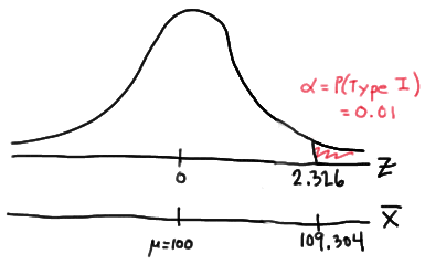
because:
\(\bar{x} = \mu + z \left( \frac{\sigma}{\sqrt{n}} \right) =100 + 2.326\left( \frac{16}{\sqrt{16}} \right)=109.304 \)
That means that the probability of rejecting the null hypothesis, when \(\mu=108\) is 0.3722 as calculated here:

So, the power when \(\mu=108\) and \(\alpha=0.01\) is smaller (0.3722) than the power when \(\mu=108\) and \(\alpha=0.05\) (0.6406)! Perhaps we can see this graphically:
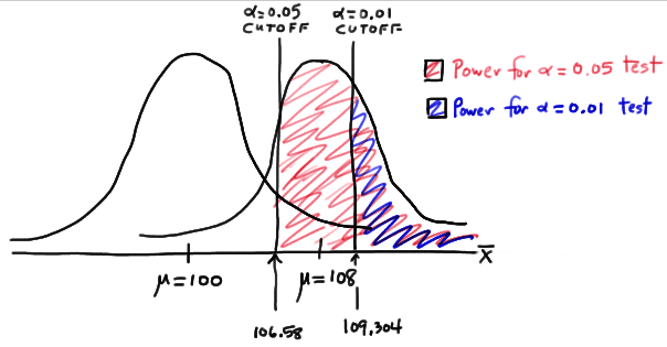
By the way, we could again alternatively look at the glass as being half-empty. In that case, the probability of a Type II error when \(\mu=108\) and \(\alpha=0.01\) is \(1-0.3722=0.6278\). In this case, the probability of a Type II error is greater than the probability of a Type II error when \(\mu=108\) and \(\alpha=0.05\).
All of this can be seen graphically by plotting the two power functions, one where \(\alpha=0.01\) and the other where \(\alpha=0.05\), simultaneously. Doing so, we get a plot that looks like this:
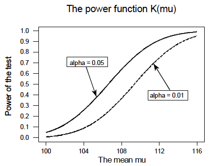
This last example illustrates that, providing the sample size \(n\) remains unchanged, a decrease in \(\alpha\) causes an increase in \(\beta\), and at least theoretically, if not practically, a decrease in \(\beta\) causes an increase in \(\alpha\). It turns out that the only way that \(\alpha\) and \(\beta\) can be decreased simultaneously is by increasing the sample size \(n\).