27.2 - The T-Test For One Mean

Answer

Our unrestricted parameter space is:

\( \Omega = \left\{ (\mu, \sigma^2) : -\infty < \mu < \infty, 0 < \sigma^2 < \infty \right\} \)

Under the null hypothesis, the mean \(\mu\) is the only parameter that is restricted. Therefore, our parameter space under the null hypothesis is:

\( \omega = \left\{(\mu, \sigma^2) : \mu =\mu_0, 0 < \sigma^2 < \infty \right\}\)

Now, first consider the case where the mean and variance are unrestricted. We showed back when we studied maximum likelihood estimation that the maximum likelihood estimates of \(\mu\) and \(\sigma^2\) are, respectively:

\(\hat{\mu} = \bar{x} \text{ and } \hat{\sigma}^2 = \dfrac{1}{n}\sum_{i=1}^{n}(x_i - \bar{x})^2 \)

Therefore, the maximum of the likelihood function for the unrestricted parameter space is:

which simplifies to:

\( L(\hat{\Omega})= \left[\dfrac{ne^{-1}}{2\pi \Sigma (x_i - \bar{x})^2} \right]^{n/2} \)

Now, under the null parameter space, the maximum likelihood estimates of \(\mu\) and \(\sigma^2\) are, respectively:

\( \hat{\mu} = \mu_0 \text{ and } \hat{\sigma}^2 = \dfrac{1}{n}\sum_{i=1}^{n}(x_i - \mu_0)^2 \)

Therefore, the likelihood under the null hypothesis is:

which simplifies to:

\( L(\hat{\omega})= \left[\dfrac{ne^{-1}}{2\pi \Sigma (x_i - \mu_0)^2} \right]^{n/2} \)

And now taking the ratio of the two likelihoods, we get:

which reduces to:

\( \lambda = \left[ \dfrac{\sum_{i=1}^{n}(x_i - \bar{x})^2}{\sum_{i=1}^{n}(x_i - \mu_0)^2} \right] ^{n/2}\)

Focusing only on the denominator for a minute, let's do that trick again of "adding 0" in just the right away. Adding 0 to the quantity in the parentheses, we get:

which simplifies to:

\( \sum_{i=1}^{n}(x_i - \mu_0)^2 = \sum_{i=1}^{n}(x_i - \bar{x})^2 +n(\bar{x} - \mu_0)^2 \)

Then, our likelihood ratio \(\lambda\) becomes:

\( \lambda = \left[ \dfrac{\sum_{i=1}^{n}(x_i - \bar{x})^2}{\sum_{i=1}^{n}(x_i - \mu_0)^2} \right] ^{n/2} = \left[ \dfrac{\sum_{i=1}^{n}(x_i - \bar{x})^2}{ \sum_{i=1}^{n}(x_i - \bar{x})^2 +n(\bar{x} - \mu_0)^2} \right] ^{n/2} \)

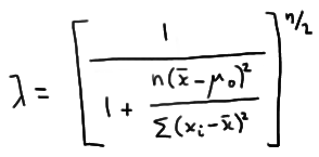
which, upon dividing through numerator and denominator by \( \sum_{i=1}^{n}(x_i - \bar{x})^2 \) simplifies to:

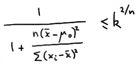
Therefore, the likelihood ratio test's critical region, which is given by the inequality \(\lambda ≤ k\), is equivalent to:

which with some minor algebraic manipulation can be shown to be equivalent to:

So, in a nutshell, we've shown that the likelihood ratio test tells us that for this situation we should reject the null hypothesis \(H_0: \mu= \mu_0\) in favor of the alternative hypothesis \(H_A: \mu ≠ \mu_0\) if:

\( \dfrac{(\bar{x}-\mu_0)^2 }{s^2 / n} \ge k^{*} \)

Well, okay, so I started out this page claiming that the t-test for a mean \(\mu\) is the likelihood ratio test. Is it? Well, the above critical region is equivalent to rejecting the null hypothesis if:

\( \dfrac{|\bar{x}-\mu_0| }{s / \sqrt{n}} \ge k^{**} \)

Does that look familiar? We previously learned that if \(X_1, X_2, \dots, X_n\) are normally distributed with mean \(\mu\) and variance \(\sigma^2\), then:

\( T = \dfrac{\bar{X}-\mu}{S / \sqrt{n}} \)

follows a T distribution with n − 1 degrees of freedom. So, this tells us that we should use the T distribution to choose \(k^{**}\). That is, set:

\(k^{**} = t_{\alpha /2, n-1}\)

and we have our size \(\alpha\) t-test that ensures the probability of committing a Type I error is \(\alpha\).