21.1 - The Run Test
21.1 - The Run TestLet's start from the beginning... it seems reasonable to think that before we can derive a Run Test, we better know what actually constitutes a run.
What is a run?
Let's suppose we have \(n_1\) observations of the random variable X, and \(n_2\) observations of the random variable Y. Suppose we combine the two sets of independent observations into one larger collection of \(n_1 + n_2\) observations, and then arrange the observations in increasing order of magnitude. If we label from which set each of the ordered observations originally came, we might observe something like this:

where x denotes an observation of the random variable X and y denotes an observation of the random variable Y. (We might observe this, for example, if the X values were 0.1, 0.4, 0.5, 0.6, 0.8, and 0.9, and the Y values were 0.2, 0.3, 0.7, 1.0, 1.1, and 1.2). That is, in this case, the smallest of all of the observations is an X value, the second smallest of all of the observations is a Y value, the third smallest of all of the observations is a Y value, the fourth smallest of all of the observations is an X value, and so on. Now, each group of successive values of X and Y is what we call a run. So, in this example, we have six runs. If we instead observed this ordered arrangement:

we would have three runs. And, if we instead observed this ordered arrangement:

we would have eight runs.
Why runs?
The next obvious question is in what way might knowing the number of runs be helpful in testing the null hypothesis of the equality of the distributions F(x) and G(y). Let's investigate that question by taking a look at a few examples. Let's start with the case in which the distributions are equal. In that case, we might observe something like this:
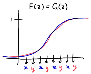
In this particular example, there are eight runs. As you can see, this kind of a picture suggests that when the distributions are equal, the number of runs will likely be large.
Now, let's take a look at one way in which the distribution functions could be unequal. One possibility is that one of the distribution functions is at least as great as the other distribution function at all points z. This situation might look something like this:
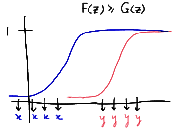
In this particular example, there are only two runs. This kind of a situation suggests that when one of the distribution functions is at least as great as the other distribution function, the number of runs will likely be small. Note that this is what the distribution functions might look like if the median of Y was greater than the median of X.
Here's another way in which the distribution functions could be unequal:
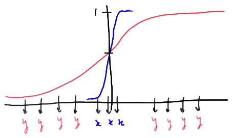
In this case, the medians of X and Y are nearly equal, but the variance of Y is much greater than the variance of X. In this particular example, there are only three runs. Again, in general, when we have this type of situation, we would expect the number of runs to be small.
The above three examples give a pretty clear indication that we're onto something with the idea of using runs to test the null hypothesis of the equality of two distribution functions. If the number of runs is smaller than expected, it seems we should reject the null hypothesis, because a small number of runs suggests that there are differences in either the location or the spread of the two distributions. Now, as is usually the case when conducting a hypothesis test, in order to quantify "smaller than expected," we're going to need to know something about the distribution of R, the number of runs.
What is the p.m.f. of R?
Let's let the random variable R denote the number of runs in the combined ordered sample containing \(n_1\) observations of X and \(n_2\) observations of Y. With possible values, such as 2, 3, and so on, R is clearly discrete. Now, if the null hypothesis is true, that is, the distribution functions are equal, all of the possible permutations of the X's and the Y's in the combined sample are equally likely. Therefore, we can use the classical approach to assigning the probability that R equals a particular value r. That is, to find the distribution of R, we can find:

for all of the possible values in the support of R. (Note that the support depends on the number of observations in the combined sample. We do know, however, that R must be at least 2.) As is usually the case, the denominator is the easy part. If we have \(n_1 + n_2\) positions:

in which we can choose to place the \(n_1\) observed x values, then the total number of ways of arranging the x's and y's is:
\(\binom{n_1+n_2}{n_1}\)
Note that once the x values are placed in their positions, the remaining \(n_2\) positions must contain the y values. We just as easily could place the y values first, and then the remaining \(n_1\) positions must contain the x values.
Now for the numerator. That's the messy part! Before we even begin to attempt to generalize a formula for the quantity in the numerator, it might be best to take a look at a concrete example.
Example 21-1

Suppose we have \(n_1 = 3\) observations of the random variable X and \(n_2 = 3\) observations of the random variable Y. What is the p.m.f. of R, the number of runs?
Answer
Put your seatbelt on. If not your seatbelt, then at least your bookkeeping hat. This is going to get a bit messy at times. So... let's start with the easy part first... the denominator! If we combine the two samples, we have a total of 3+3 = 6 observations to arrange. Therefore, there are:
\(\binom{3+3}{3}=\binom{6}{3}=\dfrac{6!}{3! 3!}=20\)
possible ways of arranging the x's and y's. Now, that's a small enough number that we can actually enumerate all 20 of the possible arrangements. Here they are:
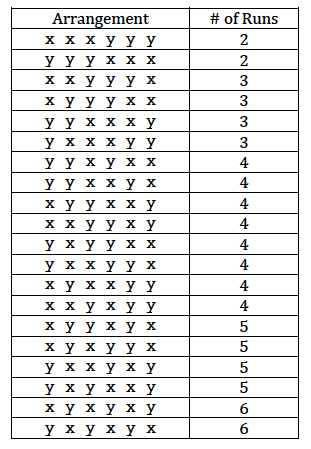
Now, as the above table suggests, of the 20 possible arrangements, there are two ways of getting R = 2 runs. Therefore:
\(P(R=2)=\frac{2}{20}\)
And, of the 20 possible arrangements, there are four ways of getting R = 3 runs. Therefore:
\(P(R=3)=\frac{4}{20}\)
Piece of cake! What was all this talk about messy bookkeeping? With the snap of a finger, we can determine the entire p.m.f. of R:

Note that the probabilities add to 1. That's a good sign! But finding the specific p.m.f. of R was not the point of this example. We were going to use this example to try to learn something about finding the p.m.f. of R in general. The only reason why we were able to find this p.m.f. of R with such ease was because we could enumerate all 20 of the possible outcomes. What if we can't do that? That is, what if there were so many possible arrangements that it would be crazy to try to enumerate them all? Well, we would go way back to what we did in Stat 414... we would derive a general counting formula! That's what we're working towards here.
Let's take a look at a case in which r is even, \(r = 4\), say. If you think about it, the only way we can get four runs is if the \(n_1 = 3\) values of X are broken up into 2 runs, which can be done in either of two ways:
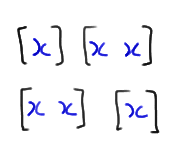
and the \(n_2 = 3\) values of Y are broken up into 2 runs, which can be done in either of two ways:
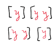
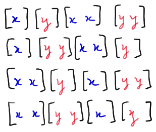
Now, it's just a matter of putting the 2 runs of X and the 2 runs of Y together to make a total of 4 runs in the sequence. Well, there are two ways of getting 2 runs of X and two ways of getting 2 runs of Y. Therefore, the multiplication rule tells us that we should expect there to be 2×2 = 4 ways of getting four runs when the samples are combined. There's just one problem with that calculation, namely that there are 2 ways of starting the sequence off. That is, we could start with an X run:
or we could start with a Y run:
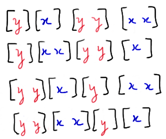
So, the multiplication rule actually tells us that there are \(2 \time 2 \times 2 = 8\) ways of getting four runs when we have \(n_1 = 3\) values of X and \(n_2 = 3\) values of Y. And, we've just enumerated all eight of them!
Now, let's try to generalize the above process. We started by considering a case in which r was even, specifically, r = 4. Note that r is even implies that \(r = 2k\), for a positive integer k. (If \(r = 4\), for example, then \(k = 2\).) Now, the only way we can get \(r = 4\) runs is if the \(n_1 = 3\) values of X are broken up into \(k = 2\) runs and the \(n_2 = 3\) values of Y are broken up into k = 2 runs. We can form the k = 2 runs of the \(n_1 = 3\) values of X by inserting \(k−1 = 1\) divider into the \(n_1 − 1 = 2\) spaces between the X values:
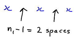
When the divider is here:

we create these two runs:

And, when the divider is here:

we create these two runs:

Note that, in general, there are:
\(\binom{n_1-1}{k-1}\)
ways of inserting k−1 dividers into the \(n_1 − 1\) spaces between the X values, with no more than one divider per space.
Now, we can go through the exact same process for the Y values. It shouldn't be too hard to see that, in general, there are:
\(\binom{n_2-1}{k-1}\)
ways of inserting k−1 dividers into the \(n_2 − 1\) spaces between the Y values, with no more than one divider per space.
Now, if you go back and look, once we broke up the X values into k = 2 runs, and the Y values into k = 2 runs, the next thing we did was to put the two sets of two runs of X and two sets of two runs of Y together. The multiplication rule tells us that there are:
\(\binom{n_1-1}{k-1}\binom{n_2-1}{k-1}\)
ways of putting the two sets of runs together to form \(r = 2k\) runs beginning with a run of x's. And, the multiplication rule tells us that there are:
\(\binom{n_2-1}{k-1}\binom{n_1-1}{k-1}\)
ways of putting the two sets of runs together to form \(r = 2k\) runs beginning with a run of y's. Therefore, the total number of ways of getting \(r = 2k\) runs is:
\(\binom{n_1-1}{k-1}\binom{n_2-1}{k-1}+\binom{n_2-1}{k-1}\binom{n_1-1}{k-1}=2\binom{n_1-1}{k-1}\binom{n_2-1}{k-1}\)
And, therefore putting the numerator and the denominator together, we get:
\(P(R=2k)=\frac{2\binom{n_1-1}{k-1}\binom{n_2-1}{k-1}}{\binom{n_1+n_2}{n_1}}\)
when k is a positive integer.
Whew! Now, we've found the probability of getting r runs when r is even. What happens if r is odd? That is, what happens if \(r = 2k+1\) for a positive integer k? Well, let's consider the case in which \(r = 3\), and therefore \(k = 1\). If you think about it, there are two ways we can get three runs... either we need \(k+1 = 2\) runs of x's and k = 1 run of y's, such as:
 and
and 
or we need \(k = 1\) run of x's and \(k+1 = 2\) runs of y's:
 and
and 
Perhaps you can see where this is going? In general, we can form \(k+1\) runs of the \(n_1\) values of X by inserting k dividers into the \(n_1−1\) spaces between the X values, with no more than one divider per space, in:
\(\binom{n_1-1}{k}\)
ways. Similarly, we can form k runs of the \(n_2\) values of Y in:
\(\binom{n_2-1}{k-1}\)
ways. The two sets of runs can be placed together to form \(2k+1\) runs in:
\(\binom{n_1-1}{k}\binom{n_2-1}{k-1}\)
ways. Likewise, \(k+1\) runs of the \(n_2\) values of Y, and k runs of the \(n_1\) values of X can be placed together to form:
\(\binom{n_2-1}{k}\binom{n_1-1}{k-1}\)
sets of \(2k+1\) runs. Therefore, the total number of ways of getting \(r = 2k+1\) runs is:
\(\binom{n_1-1}{k}\binom{n_2-1}{k-1}+\binom{n_2-1}{k}\binom{n_1-1}{k-1}\)
And, therefore putting the numerator and the denominator together, we get:
\(P(R=2k+1)=\frac{\binom{n_1-1}{k}\binom{n_2-1}{k-1}+\binom{n_2-1}{k}\binom{n_1-1}{k-1}}{\binom{n_1+n_2}{n_1}} \)
Yikes! Let's put this example to rest!
Let's summarize what we've learned.
Summary. The probability that R, the number of runs, takes on a particular value r is:
\(P(R=2k)=\dfrac{2\binom{n_1-1}{k-1}\binom{n_2-1}{k-1}}{\binom{n_1+n_2}{n_1}}\)
if r is even, that is, if \(r = 2k\) for a positive integer k. The probability that R, the number of runs, takes on a particular value r is:
\(P(R=2k+1)=\dfrac{\binom{n_1-1}{k}\binom{n_2-1}{k-1}+\binom{n_2-1}{k}\binom{n_1-1}{k-1}}{\binom{n_1+n_2}{n_1}} \)
if r is odd, that is, if\(r = 2k + 1\) for a positive integer k.
Now, let's wrap up our development of the Run Test with an example.
Example 21-2

Let X and Y denote the times in hours per weeks that students in two different schools watch television. Let F(x) and G(y) denote the respective distributions. To test the null hypothesis:
\(H_0 : F(z) =G(z)\)
a random sample of eight students was selected from each school, yielding the following results:

What conclusion should we make about the equality of the two distribution functions?
Answer
The combined ordered sample, with the x values in blue and the y values in red, looks like this:

Counting, we see that there are 9 runs. We should reject the null hypothesis if the number of runs is smaller than expected. Therefore, the critical region should be of the form r ≤ c. In order to determine what we should set the value of c to be, we'll need to know something about the p.m.f. of R. We can use the formulas that we derived above to determine various probabilities. Well, with \(n_1 = 8 , n_2 = 8 , \text{ and } k = 1\), we have:
\(P(R=2)=\dfrac{2\binom{7}{0}\binom{7}{0}}{\binom{16}{8}}=\dfrac{2}{12,870}=0.00016\)
and:
\(P(R=3)=\dfrac{\binom{7}{1}\binom{7}{0}+\binom{7}{1}\binom{7}{0}}{\binom{16}{8}}=\dfrac{14}{12,870}=0.00109\)
(Note that Table I in the back of the textbook can be helpful in evaluating the value of the "binomial coefficients.") Now, with \(n_1 = 8 , n_2 = 8 , \text{ and } k = 2\), we have:
\(P(R=4)=\dfrac{2\binom{7}{1}\binom{7}{1}}{\binom{16}{8}}=\dfrac{98}{12,870}=0.00761\)
and:
\(P(R=5)=\dfrac{\binom{7}{2}\binom{7}{1}+\binom{7}{2}\binom{7}{1}}{\binom{16}{8}}=\dfrac{294}{12,870}=0.02284\)
And, with \(n_1 = 8 , n_2 = 8 , \text{ and } k = 3\), we have:
\(P(R=6)=\dfrac{2\binom{7}{2}\binom{7}{2}}{\binom{16}{8}}=\dfrac{882}{12,870}=0.06853\)
Let's stop to see what we have going for us so far. Well, so far we've learned that:
\(P(R \le 6)=0.00016+0.00109+0.00761+0.02284+0.06853=0.1002\)
Hmmm. That tells us that if we set c = 6, we'd have a 0.1002 probability of committing a Type I error. That seems reasonable! That is, let's decide to reject the null hypothesis of the equality of the two distribution functions if the number of observed runs \(r ≤ 6\). It's not... we observed 9 runs. Therefore, we fail to reject the null hypothesis at the 0.10 level. There is insufficient evidence at the 0.10 level to conclude that the distribution functions are not equal.
A Large-Sample Test
As our work in the previous example illustrates, conducting a single run test can be quite extensive in the calculation front. Is there an easier way? Fortunately, yes... that is, providing \(n_1\) and \(n_2\) are large. Typically, we consider the samples to be large if \(n_1\) is at least 10 and \(n_2\) is at least 10. If the samples are large, then the distribution of R can be approximated with a normally distributed random variable. That is, it can be shown that:
\(Z=\dfrac{R-\mu_R}{\sqrt{Var(R)}}\)
follows an approximate standard normal \(N(0, 1)\) distribution with mean:
\(\mu_R=E(R)=\dfrac{2n_1n_2}{n_1+n_2}+1 \)
and variance:
\( Var(R)=\dfrac{2n_1n_2(2n_1n_2-n_1-n_2)}{(n_1+n_2)^2(n_1+n_2-1)}\).
Because a small number of runs is evidence that the distribution functions are unequal, the critical region for testing the null hypothesis:
\(H_0 : F(z) = G(z)\)
is of the form \(z ≤ −z_{\alpha}\), where \(\alpha\) is the desired significance level. Let's take a look at an example.
Example 21-3

A charter bus line has 48-passenger buses and 38-passenger buses. With X and Y denoting the number of miles traveled per day for the 48-passenger and 38-passenger buses, respectively, the bus company is interested in testing the equality of the two distributions:
\(H_0 : F(z) = G(z)\)
The company observed the following data on a random sample of \(n_1 = 10\) buses holding 48 passengers and \(n_2 = 11\) buses holding 38 passengers:

Using the normal approximation to R, conduct the hypothesis test at the 0.05 level.
Answer
The combined ordered sample, with the x values in blue and the y values in red, looks like this:

Counting, we see that there are 9 runs. Using the normal approximation to R, with \(n_1 = 10\) and \(n_2 = 11\), we have:
\(\mu_R=\dfrac{2n_1n_2}{n_1+n_2}+1=\dfrac{2(10)(11)}{10+11}+1=11.476\)
and:
\( Var(R)=\dfrac{2n_1n_2(2n_1n_2-n_1-n_2)}{(n_1+n_2)^2(n_1+n_2-1)} =\dfrac{2(10)(11)[2(10)(11)-10-11]}{(10+11)^2(10+11-1)}=4.9637\)
Now, we observed r = 9 runs. Therefore, the approximate P-value, using a half-unit correction for continuity, is:
\(P \approx P\left[Z \le \dfrac{9.5-11.476}{\sqrt{4.9637}} \right]=P[Z \le -0.89]=0.187\)
We fail to reject the null hypothesis at the 0.05 level, because the P-value is greater than 0.05. There is insufficient evidence at the 0.05 level to conclude that the two distribution functions are unequal.