Lesson 3: Probability Distributions
Lesson 3: Probability DistributionsOverview
In this Lesson, we take the next step toward inference. In Lesson 2, we introduced events and probability properties. In this Lesson, we will learn how to numerically quantify the outcomes into a random variable. Then we will use the random variable to create mathematical functions to find probabilities of the random variable.
One of the most important discrete random variables is the binomial distribution and the most important continuous random variable is the normal distribution. They will both be discussed in this lesson. We will also talk about how to compute the probabilities for these two variables.
Objectives
- Distinguish between discrete and continuous random variables.
- Compute probabilities, cumulative probabilities, means and variances for discrete random variables.
- Identify binomial random variables and their characteristics.
- Calculate probabilities of binomial random variables.
- Describe the properties of the normal distribution.
- Find probabilities and percentiles of any normal distribution.
- Apply the Empirical rule.
3.1 - Random Variables
3.1 - Random VariablesWhat is a random variable?
Let's use a scenario to introduce the idea of a random variable.
Suppose we flip a fair coin three times and record if it shows a head or a tail. The outcome or sample space is S={HHH,HHT,HTH,THH,TTT,TTH,THT,HTT}. There are eight possible outcomes and each of the outcomes is equally likely. Now, suppose we flipped a fair coin four times. How many possible outcomes are there? There are $2^4 = 16$. How about ten times? $1024$ possible outcomes! Instead of considering all the possible outcomes, we can consider assigning the variable $X$, say, to be the number of heads in $n$ flips of a fair coin. If we flipped the coin $n=3$ times (as above), then $X$ can take on possible values of \(0, 1, 2,\) or \(3\). By defining the variable, \(X\), as we have, we created a random variable.
- Random Variable
-
A random variable is a variable that takes on different values determined by chance. In other words, it is a numerical quantity that varies at random.
Types of Random Variables
There are mainly two types of random variables:
- Discrete Random Variable
- When the random variable can assume only a countable, sometimes infinite, number of values.
- Continuous Random Variable
- When the random variable can assume an uncountable number of values in a line interval.
Probability Functions
Transforming the outcomes to a random variable allows us to quantify the outcomes and determine certain characteristics. If we have a random variable, we can find it’s probability function.
- Probability Function
-
A probability function is a mathematical function that provides probabilities for the possible outcomes of the random variable, \(X\). It is typically denoted as \(f(x)\).
There are two classes of probability functions: Probability Mass Functions and Probability Density Functions.
- Probability Mass Function (PMF)
-
If the random variable is a discrete random variable, the probability function is usually called the probability mass function (PMF). If X is discrete, then \(f(x)=P(X=x)\). In other words, the PMF for a constant, \(x\), is the probability that the random variable \(X\) is equal to \(x\). The PMF can be in the form of an equation or it can be in the form of a table.
-
Properties of probability mass functions:
- \(f(x)>0\), for x in the sample space and 0 otherwise.
- \(\sum_x f(x)=1\). In other words, the sum of all the probabilities of all the possible outcomes of an experiment is equal to 1.
-
- Probability Density Function (PDF)
-
If the random variable is a continuous random variable, the probability function is usually called the probability density function (PDF). Contrary to the discrete case, $f(x)\ne P(X=x)$
-
Properties of a probability density function:
- \(f(x)>0\), for x in the sample space and 0 otherwise.
- The area under the curve is equal to 1.
-
The probability of a random variable being less than or equal to a given value is calculated using another probability function called the cumulative distribution function.
- Cumulative Distribution Function (CDF)
-
A cumulative distribution function (CDF), usually denoted $F(x)$, is a function that gives the probability that the random variable, X, is less than or equal to the value x.
-
\(F(x)=P(X\le x)\)
-
Note! The definition of the cumulative distribution function is the same for a discrete random variable or a continuous random variable. For a continuous random variable, however, \(P(X=x)=0\). Therefore, the CDF, \(F(x)=P(X\le x)=P(X<x)\), for the continuous case.
-
3.2 - Discrete Probability Distributions
3.2 - Discrete Probability DistributionsThis section takes a look at some of the characteristics of discrete random variables.
Consider the data set with the values: \(0, 1, 2, 3, 4\). If \(X\) is a random variable of a random draw from these values, what is the probability you select 2? If we assume the probabilities of each of the values is equal, then the probability would be \(P(X=2)=\frac{1}{5}\). We can define the probabilities of each of the outcomes using the probability mass function (PMF) described in the last section. If we assume the probabilities of all the outcomes were the same, the PMF could be displayed in function form or a table. As a function, it would look like: \(f(x)=\begin{cases} \frac{1}{5} & x=0, 1, 2, 3, 4\\ 0 & \text{otherwise} \end{cases}\)
As a table, it would look like:
| \(x\) | 0 | 1 | 2 | 3 | 4 |
|---|---|---|---|---|---|
| \(f(x)\) | 1/5 | 1/5 | 1/5 | 1/5 | 1/5 |
Recall that for a PMF, \(f(x)=P(X=x)\). In other words, the PMF gives the probability our random variable is equal to a value, x. We can also find the CDF using the PMF.
Example 3-1: CDF
Find the CDF, in tabular form of the random variable, X, as defined above.
| \(x\) | 0 | 1 | 2 | 3 | 4 |
|---|---|---|---|---|---|
| \(f(x) = P(X=x)\) | 1/5 | 1/5 | 1/5 | 1/5 | 1/5 |
Answer
Recall that \(F(X)=P(X\le x)\). Start by finding the CDF at \(x=0\).
\(F(0)=P(X\le 0)\)
Since 0 is the smallest value of \(X\), then \(F(0)=P(X\le 0)=P(X=0)=\frac{1}{5}\)
Now, find \(F(1)\).
\begin{align} F(1)=P(X\le 1)&=P(X=1)+P(X=0)\\&=\frac{1}{5}+\frac{1}{5}\\&=\frac{2}{5}\end{align}
Next, \(F(2)\).
\begin{align} F(2)=P(X\le 2)&=P(X=2)+P(X=1)+P(X=0)\\&=\frac{1}{5}+\frac{1}{5}+\frac{1}{5}\\&=\frac{3}{5}\end{align}
Next, \(F(3)\).
\begin{align} F(3)=P(X\le 3)&=P(X=3)+P(X=2)+P(X=1)+P(X=0)\\&=\frac{1}{5}+\frac{1}{5}+\frac{1}{5}+\frac{1}{5}\\&=\frac{4}{5}\end{align}
Finally, \(F(4)\).
\begin{align} F(4)=P(X\le 4)&=P(X=4)+P(X=3)+P(X=2)+P(X=1)+P(X=0)\\&=\frac{1}{5}+\frac{1}{5}+\frac{1}{5}+\frac{1}{5}+\frac{1}{5}\\&=\frac{5}{5}=1\end{align}
In table form...
| \(x\) | 0 | 1 | 2 | 3 | 4 |
|---|---|---|---|---|---|
| \(F(x) = P(X\le x)\) | 1/5 | 2/5 | 3/5 | 4/5 | 5/5=1 |
This table provides the probability of each outcome and those prior to it. Thus, the probability for the last event in the cumulative table is 1 since that outcome or any previous outcomes must occur.
Try It!
Use the table from the example above to answer the following questions.
| \(x\) | 0 | 1 | 2 | 3 | 4 |
|---|---|---|---|---|---|
| \(f(x) = P(X=x)\) | 1/5 | 1/5 | 1/5 | 1/5 | 1/5 |
-
Find \(P(X=1)\)
\(P(X=1)=\dfrac{1}{5}\)
-
Find \(P(X\le 2)\)\begin{align} P(X\le 2)&=P(X=0)+P(X=1)+P(X=2)\\&=\dfrac{1}{5}+\dfrac{1}{5}+\dfrac{1}{5}\\&=\dfrac{3}{5}\end{align}
-
\(P(X<3)\)
\(P(X<3)=P(X\le 2)=\dfrac{3}{5}\). Note that \(P(X<3)\) does not equal \(P(X\le 3)\) as it does not include \(P(X=3)\).
-
\(P(1\le X\le 3)\)\(P(1\le X\le 3)=P(X=1)+P(X=2)+P(X=3)=\dfrac{3}{5}\)
3.2.1 - Expected Value and Variance of a Discrete Random Variable
3.2.1 - Expected Value and Variance of a Discrete Random VariableBy continuing with example 3-1, what value should we expect to get? What would be the average value?
We can answer this question by finding the expected value (or mean).
- Expected Value (or mean) of a Discrete Random Variable
-
For a discrete random variable, the expected value, usually denoted as \(\mu\) or \(E(X)\), is calculated using:
-
\(\mu=E(X)=\sum x_if(x_i)\)
- The formula means that we multiply each value, \(x\), in the support by its respective probability, \(f(x)\), and then add them all together. It can be seen as an average value but weighted by the likelihood of the value.
-
Example 3-2: Expected Value
In Example 3-1 we were given the following discrete probability distribution:
| \(x\) | 0 | 1 | 2 | 3 | 4 |
|---|---|---|---|---|---|
| \(f(x)\) | 1/5 | 1/5 | 1/5 | 1/5 | 1/5 |
What is the expected value?
Answer
\begin{align} \mu=E(X)=\sum xf(x)&=0\left(\frac{1}{5}\right)+1\left(\frac{1}{5}\right)+2\left(\frac{1}{5}\right)+3\left(\frac{1}{5}\right)+4\left(\frac{1}{5}\right)\\&=2\end{align}
For this example, the expected value was equal to a possible value of X. This may not always be the case. For example, if we flip a fair coin 9 times, how many heads should we expect? We will explain how to find this later but we should expect 4.5 heads. The expected value in this case is not a valid number of heads.
Now that we can find what value we should expect, (i.e. the expected value), it is also of interest to give a measure of the variability.
- Variance of a Discrete Random Variable
-
The variance of a discrete random variable is given by:
-
\(\sigma^2=\text{Var}(X)=\sum (x_i-\mu)^2f(x_i)\)
-
The formula means that we take each value of x, subtract the expected value, square that value and multiply that value by its probability. Then sum all of those values.
There is an easier form of this formula we can use.
\(\sigma^2=\text{Var}(X)=\sum x_i^2f(x_i)-E(X)^2=\sum x_i^2f(x_i)-\mu^2\)
The formula means that first, we sum the square of each value times its probability then subtract the square of the mean. We will use this form of the formula in all of our examples.
-
- Standard Deviation of a Discrete Random Variable
-
The standard deviation of a random variable, $X$, is the square root of the variance.
- \(\sigma=\text{SD}(X)=\sqrt{\text{Var}}(X)=\sqrt{\sigma^2}\)
Example 3-3: Standard Deviation
Consider the first example where we had the values 0, 1, 2, 3, 4. The PMF in tabular form was:
| \(x\) | 0 | 1 | 2 | 3 | 4 |
|---|---|---|---|---|---|
| \(f(x)\) | 1/5 | 1/5 | 1/5 | 1/5 | 1/5 |
Find the variance and the standard deviation of X.
Answer
\(\text{Var}(X)=\left[0^2\left(\dfrac{1}{5}\right)+1^2\left(\dfrac{1}{5}\right)+2^2\left(\dfrac{1}{5}\right)+3^2\left(\dfrac{1}{5}\right)+4^2\left(\dfrac{1}{5}\right)\right]-2^2=6-4=2\)
\(\text{SD}(X)=\sqrt{2}\approx 1.4142\)
Example 3-4: Prior Convictions
Click on the tab headings to see how to find the expected value, standard deviation, and variance. The last tab is a chance for you to try it.

Let X = number of prior convictions for prisoners at a state prison at which there are 500 prisoners. (\(x = 0,1,2,3,4\))
| \(X=x\) | 0 | 1 | 2 | 3 | 4 |
|---|---|---|---|---|---|
| \(Number\ of\ Prisoners\) | 80 | 265 | 100 | 40 | 15 |
| \(f(x) = P(X=x)\) | 80/500 | 265/500 | 100/500 | 40/500 | 15/500 |
| \(f(x)=P(X=x)\) | 0.16 | 0.53 | 0.2 | 0.08 | 0.03 |
What is the expected value for number of prior convictions?
| \(X=x\) | 0 | 1 | 2 | 3 | 4 |
|---|---|---|---|---|---|
| \(Number\ of\ Prisoners\) | 80 | 265 | 100 | 40 | 15 |
| \(f(x) = P(X=x)\) | 80/500 | 265/500 | 100/500 | 40/500 | 15/500 |
| \(f(x)=P(X=x)\) | 0.16 | 0.53 | 0.2 | 0.08 | 0.03 |
Answer
For this we need a weighted average since not all the outcomes have equal chance of happening (i.e. they are not equally weighted). So, we need to find our expected value of \(X\), or mean of \(X\), or \(E(X) = \Sigma f(x_i)(x_i)\). When we write this out it follows:
\(=(0.16)(0)+(0.53)(1)+(0.2)(2)+(0.08)(3)+(0.03)(4)=1.29\)
Calculate the variance and the standard deviation for the Prior Convictions example:
| \(X=x\) | 0 | 1 | 2 | 3 | 4 |
|---|---|---|---|---|---|
| \(Number\ of\ Prisoners\) | 80 | 265 | 100 | 40 | 15 |
| \(f(x) = P(X=x)\) | 80/500 | 265/500 | 100/500 | 40/500 | 15/500 |
| \(f(x)=P(X=x)\) | 0.16 | 0.53 | 0.2 | 0.08 | 0.03 |
Answer
Using the data in our example we find that...
\begin{align} \text{Var}(X) &=[0^2(0.16)+1^2(0.53)+2^2(0.2)+3^2(0.08)+4^2(0.03)]–(1.29)^2\\ &=2.53–1.66\\ &=0.87\\ \text{SD}(X) &=\sqrt(0.87)\\ &=0.93 \end{align}
What is the expected number of prior convictions? Below is the probability distribution table for the prior conviction data. Use this table to answer the questions that follow.
| \(X=x\) | 0 | 1 | 2 | 3 | 4 |
|---|---|---|---|---|---|
| \(f(x)=P(X=x)\) | 0.16 | 0.53 | 0.2 | 0.08 | 0.03 |
3.2.2 - Binomial Random Variables
3.2.2 - Binomial Random VariablesA binary variable is a variable that has two possible outcomes. For example, sex (male/female) or having a tattoo (yes/no) are both examples of a binary categorical variable.
A random variable can be transformed into a binary variable by defining a “success” and a “failure”. For example, consider rolling a fair six-sided die and recording the value of the face. The random variable, value of the face, is not binary. If we are interested, however, in the event A={3 is rolled}, then the “success” is rolling a three. The failure would be any value not equal to three. Therefore, we can create a new variable with two outcomes, namely A = {3} and B = {not a three} or {1, 2, 4, 5, 6}. This new variable is now a binary variable.
Binary Categorical Variable
A binary categorical variable is a variable that has two possible outcomes.
The Binomial Distribution
The binomial distribution is a special discrete distribution where there are two distinct complementary outcomes, a “success” and a “failure”.
We have a binomial experiment if ALL of the following four conditions are satisfied:
- The experiment consists of n identical trials (n is fixed).
- Each trial results in one of the two outcomes, called success and failure.
- The probability of success, denoted p, remains the same from trial to trial.
- The n trials are independent. That is, the outcome of any trial does not affect the outcome of the others.
If the four conditions are satisfied, then the random variable \(X\)=number of successes in \(n\) trials, is a binomial random variable with
\begin{align}
&\mu=E(X)=np &&\text{(Mean)}\\
&\text{Var}(X)=np(1-p) &&\text{(Variance)}\\
&\text{SD}(X)=\sqrt{np(1-p)} \text{, where \(p\) is the probability of the “success."} &&\text{(Standard Deviation)}\\
\end{align}
A Note on Notation! Some common notation for “success” that you may see will be either \(p\) or \(\pi\) to represent the probability of “success” and usually \(q=1-p\) to represent the probability of “failure”. \(\pi\) is what is used in text. “Success” is defined as whatever the researcher decides…not just a positive outcome. The symbol \(\pi\) is this case does NOT refer the numerical value 3.14
\(p \;(or\ \pi)\) = probability of success
Example 3-5: Prior Convictions
Let's use the example from the previous page investigating the number of prior convictions for prisoners at a state prison at which there were 500 prisoners. Define the “success” to be the event that a prisoner has no prior convictions. Find \(p\) and \(1-p\).
Answer
Let Success = no priors (0)
Let Failure = priors (1, 2, 3, or 4)
Looking back on our example, we can find that:
\(p=0.16\)
\(1-p=1-0.16=0.84\)
Verify by \(p+(1-p)=1\)
Example 3-6: Crime Survey
An FBI survey shows that about 80% of all property crimes go unsolved. Suppose that in your town 3 such crimes are committed and they are each deemed independent of each other. What is the probability that 1 of 3 of these crimes will be solved?
First, we must determine if this situation satisfies ALL four conditions of a binomial experiment:
- Does it satisfy a fixed number of trials? YES the number of trials is fixed at 3 (n = 3.)
- Does it have only 2 outcomes? YES (Solved and unsolved)
- Do all the trials have the same probability of success? YES (p = 0.2)
- Are all crimes independent? YES (Stated in the description.)
To find the probability that only 1 of the 3 crimes will be solved we first find the probability that one of the crimes would be solved. With three such events (crimes) there are three sequences in which only one is solved:
- Solved First, Unsolved Second, Unsolved Third = (0.2)(0.8)( 0.8) = 0.128
- Unsolved First, Solved Second, Unsolved Third = (0.8)(0.2)(0.8) = 0.128
- Unsolved First, Unsolved Second, Solved Third = (0.8)(0.8)(0.2) = 0.128
We add these 3 probabilities up to get 0.384. Looking at this from a formula standpoint, we have three possible sequences, each involving one solved and two unsolved events. Putting this together gives us the following: \(3(0.2)(0.8)^2=0.384\)
The example above and its formula illustrates the motivation behind the binomial formula for finding exact probabilities.
The Binomial Formula
For a binomial random variable with probability of success, \(p\), and \(n\) trials...
\(f(x)=P(X = x)=\dfrac{n!}{x!(n−x)!}p^x(1–p)^{n-x}\) for \(x=0, 1, 2, …, n\)
Graphical Displays of Binomial Distributions
The formula defined above is the probability mass function, pmf, for the Binomial. We can graph the probabilities for any given \(n\) and \(p\). The following distributions show how the graphs change with a given n and varying probabilities.
Example 3-7: Crime Survey Continued...
For the FBI Crime Survey example, what is the probability that at least one of the crimes will be solved?
Answer
Here we are looking to solve \(P(X \ge 1)\).
There are two ways to solve this problem: the long way and the short way.
The long way to solve for \(P(X \ge 1)\). This would be to solve \(P(x=1)+P(x=2)+P(x=3)\) as follows:
\(P(x=1)=\dfrac{3!}{1!2!}0.2^1(0.8)^2=0.384\)
\(P(x=2)=\dfrac{3!}{2!1!}0.2^2(0.8)^1=0.096\)
\(P(x=3)=\dfrac{3!}{3!0!}0.2^3(0.8)^0=0.008\)
We add up all of the above probabilities and get 0.488...OR...we can do the short way by using the complement rule. Here the complement to \(P(X \ge 1)\) is equal to \(1 - P(X < 1)\) which is equal to \(1 - P(X = 0)\). We have carried out this solution below.
\begin{align} 1–P(x<1)&=1–P(x=0)\\&=1–\dfrac{3!}{0!(3−0)!}0.2^0(1–0.2)^3\\ &=1−1(1)(0.8)^3\\ &=1–0.512\\ &=0.488 \end{align}
In such a situation where three crimes happen, what is the expected value and standard deviation of crimes that remain unsolved? Here we apply the formulas for expected value and standard deviation of a binomial.
\begin{align} \mu &=E(X)\\ &=3(0.8)\\ &=2.4 \end{align} \begin{align} \text{Var}(X)&=3(0.8)(0.2)=0.48\\ \text{SD}(X)&=\sqrt{0.48}\approx 0.6928 \end{align}
Note: X can only take values 0, 1, 2, ..., n, but the expected value (mean) of X may be some value other than those that can be assumed by X.
Example 3-8: Cross-Fertilizing
Cross-fertilizing a red and a white flower produces red flowers 25% of the time. Now we cross-fertilize five pairs of red and white flowers and produce five offspring. Find the probability that there will be no red-flowered plants in the five offspring.
Answer
Y = # of red flowered plants in the five offspring. Here, the number of red-flowered plants has a binomial distribution with \(n = 5, p = 0.25\).
\begin{align} P(Y=0)&=\dfrac{5!}{0!(5−0)!}p^0(1−p)^5\\&=1(0.25)^0(0.75)^5\\&=0.237 \end{align}
Try it!
Refer to example 3-8 to answer the following.
- Find the probability that there will be four or more red-flowered plants.
\begin{align} P(\mbox{Y is 4 or more})&=P(Y=4)+P(Y=5)\\ &=\dfrac{5!}{4!(5-4)!} {p}^4 {(1-p)}^1+\dfrac{5!}{5!(5-5)!} {p}^5 {(1-p)}^0\\ &=5\cdot (0.25)^4 \cdot (0.75)^1+ (0.25)^5\\ &=0.015+0.001\\ &=0.016\\ \end{align}
- Of the five cross-fertilized offspring, how many red-flowered plants do you expect?\begin{align} \mu &=5⋅0.25\\&=1.25 \end{align}
- What is the standard deviation of Y, the number of red-flowered plants in the five cross-fertilized offspring?\begin{align} \sigma&=\sqrt{5\cdot0.25\cdot0.75}\\ &=0.97 \end{align}
3.2.3 - Minitab: Binomial Distributions
3.2.3 - Minitab: Binomial DistributionsMinitab® – Finding Binomial Probabilities using Minitab
Let’s walk through how to calculate the probability of 1 out of 3 crimes being solved in the FBI Crime Survey example.
Recall in that example, \(n=3\), \(p=0.2\).
Using Minitab, calculate \(P(X=1)\):
- From the Minitab menu select Calc > Probability Distributions > Binomial
- A dialog box (below) will appear. Enter 3 into the Number of Trials box and 0.2 into the Event Probability box.
- Choose Probability .
- Choose the Input Constant Box and enter 1.
- Choose OK .
The result should be the same probability of 0.384 we found by hand.
Suppose we want to find \(P(X\le 2)\). We can use Minitab to find this cumulative probability.
- From the Minitab menu select Calc > Probability Distributions > Binomial
- Enter in 3 and 0.2 as above.
- Choose Cumulative Probability .
- Choose Input Constant and enter 2.
- Choose OK .
The result should be \(P(X\le 2)=0.992\).
Note!
Depending on if you have the desktop version or cloud version of MINITAB, you will find minor differences in the order of the steps.
Binomial with Minitab
Suppose X follows a binomial distribution with 𝑛=3 and 𝑝=0.2. Calculate 𝑃(𝑋=1).
Calc > Probability Distributions > Probability Density. Fill the dialog box as shown below.
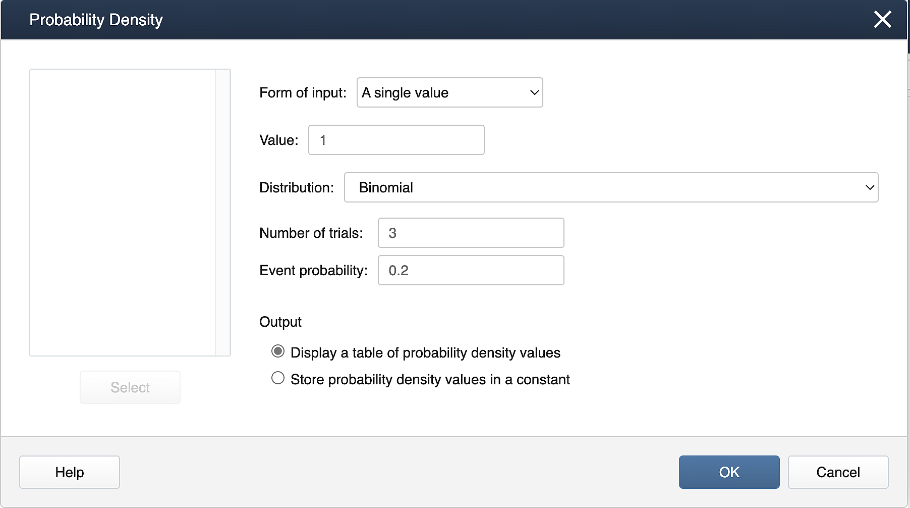
Binomial with n= 3 and p = 0.2
x
P(X=x)
1
0.383
Suppose X follows a binomial distribution with 𝑛=3 and 𝑝=0.2. Calculate P(𝑋≤2).
Calc > Probability Distributions > Cumulative Distribution Function. Fill the dialog box as shown below.
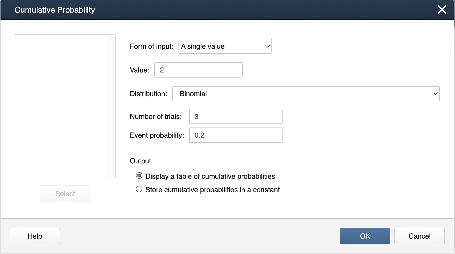
Binomial with n= 3 and p = 0.2
x
P(X≤x)
2
0.992
3.3 - Continuous Probability Distributions
3.3 - Continuous Probability DistributionsOverview
In the beginning of the course we looked at the difference between discrete and continuous data. The last section explored working with discrete data, specifically, the distributions of discrete data. In this lesson we're again looking at the distributions but now in terms of continuous data. Examples of continuous data include...
- the amount of rainfall in inches in a year for a city.
- the weight of a newborn baby.
- the height of a randomly selected student.
Properties of Continuous Probability Functions
At the beginning of this lesson, you learned about probability functions for both discrete and continuous data. Recall that if the data is continuous the distribution is modeled using a probability density function ( or PDF).
We define the probability distribution function (PDF) of \(Y\) as \(f(y)\) where: \(P(a < Y < b)\) is the area under \(f(y)\) over the interval from \(a\) to \(b\). (see figure below)
To find probabilities over an interval, such as \(P(a<Y<b)\), using the pdf would require calculus. Instead of doing the calculations by hand, we rely on software and tables to find these probabilities.
Expected value and Variance of a Continuous Random Variable
The expected value and the variance have the same meaning (but different equations) as they did for the discrete random variables.
- Expected Value (or mean) of a Continuous Random Variable
-
The expected value (or mean) of a continuous random variable is denoted by \(\mu=E(Y)\).
- Variance of a Continuous Random Variable
-
The variance of a continuous random variable is denoted by \(\sigma^2=\text{Var}(Y)\).
- Standard Deviation of a Continuous Random Variable
-
The standard deviation of a continuous random variable is denoted by $\sigma=\sqrt{\text{Var}(Y)}$
Notice the equations are not provided for the three parameters above. Therefore, for the continuous case, you will not be asked to find these values by hand.
There are many commonly used continuous distributions. The most important one for this class is the normal distribution. We will describe other distributions briefly.
3.3.1 - The Normal Distribution
3.3.1 - The Normal DistributionThe Normal Distribution is a family of continuous distributions that can model many histograms of real-life data which are mound-shaped (bell-shaped) and symmetric (for example, height, weight, etc.).
A normal curve has two parameters:
- mean $\mu$ (center of the curve)
- standard deviation $\sigma$ (spread about the center) (..and variance $\sigma^2$)
The mean can be any real number and the standard deviation is greater than zero. The normal curve ranges from negative infinity to infinity. The image below shows the effect of the mean and standard deviation on the shape of the normal curve.
3.3.2 - The Standard Normal Distribution
3.3.2 - The Standard Normal DistributionA special case of the normal distribution has mean \(\mu = 0\) and a variance of \(\sigma^2 = 1\). The 'standard normal' is an important distribution.
Standard Normal Distribution
A standard normal distribution has a mean of 0 and variance of 1. This is also known as a z distribution. You may see the notation \(N(\mu, \sigma^2\)) where N signifies that the distribution is normal, \(\mu\) is the mean, and \(\sigma^2\) is the variance. A Z distribution may be described as \(N(0,1)\). Note that since the standard deviation is the square root of the variance then the standard deviation of the standard normal distribution is 1.
Finding Probabilities of a Standard Normal Random Variable
As we mentioned previously, calculus is required to find the probabilities for a Normal random variable. Fortunately, we have tables and software to help us.
For any normal random variable, we can transform it to a standard normal random variable by finding the Z-score. Then we can find the probabilities using the standard normal tables.
Most statistics books provide tables to display the area under a standard normal curve. Look in the appendix of your textbook for the Standard Normal Table. We include a similar table, the Standard Normal Cumulative Probability Table so that you can print and refer to it easily when working on the homework.
Most standard normal tables provide the “less than probabilities”. For example, if \(Z\) is a standard normal random variable, the tables provide \(P(Z\le a)=P(Z<a)\), for a constant, \(a\).
Example 3-9: Probability 'less than'
Find the area under the standard normal curve to the left of 0.87.
There are two main ways statisticians find these numbers that require no calculus! Click on the tabs below to see how to answer using a table and using technology.
A typical four-decimal-place number in the body of the Standard Normal Cumulative Probability Table gives the area under the standard normal curve that lies to the left of a specified z-value. The probability to the left of z = 0.87 is 0.8078 and it can be found by reading the table:
- Since z = 0.87 is positive, use the table for POSITIVE z-values.
- Go down the left-hand column, label z to "0.8."
- Then, go across that row until under the "0.07" in the top row.
You should find the value, 0.8078. Therefore,\(P(Z< 0.87)=P(Z\le 0.87)=0.8078\)
z | .00 | .01 | .02 | .03 | .04 | .05 | .06 | .07 | .08 | .09 |
|---|---|---|---|---|---|---|---|---|---|---|
0.6 | .7257 | .7291 | .7324 | .7357 | .7389 | .7422 | .7454 | .7586 | .7517 | .7549 |
0.7 | .7580 | .7611 | .7642 | .7673 | .7704 | .7734 | .7764 | .7794 | .7823 | .7852 |
0.8 | .7881 | .7910 | .7939 | .7967 | .7995 | .8023 | .8051 | .8078 | .8106 | .8133 |
0.9 | .8159 | .8186 | .8212 | .8238 | .8264 | .8289 | .8315 | .8340 | .8365 | .8389 |
Using Minitab
To find the area to the left of z = 0.87 in Minitab...
- From the Minitab menu select Calc> Probability Distributions> Normal.
- Select Cumulative Probability.
- In the Input constant box, enter 0.87. Click OK
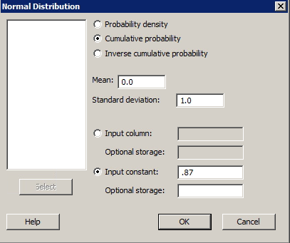
You should see a value very close to 0.8078.
Example 3-10: Probability 'greater than'
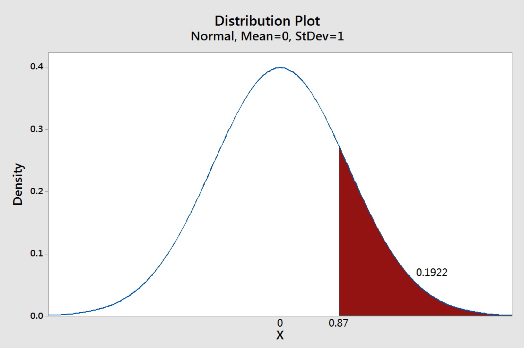
Find the area under the standard normal curve to the right of 0.87.
Based on the definition of the probability density function, we know the area under the whole curve is one. Since we are given the “less than” probabilities in the table, we can use complements to find the “greater than” probabilities. Therefore,
\(P(Z>0.87)=1-P(Z\le 0.87)\).
Using the information from the last example, we have \(P(Z>0.87)=1-P(Z\le 0.87)=1-0.8078=0.1922\)
Using Minitab
Since we are given the “less than” probabilities when using the cumulative probability in Minitab, we can use complements to find the “greater than” probabilities. Therefore,
\(P(Z>0.87)=1-P(Z\le 0.87)\).
Using the information from the last example, we have \(P(Z>0.87)=1-P(Z\le 0.87)=1-0.8078=0.1922\)
You can also use the probability distribution plots in Minitab to find the "greater than."
- Select Graph> Probability Distribution Plot> View Probability and click OK.
- In the pop-up window select the Normal distribution with a mean of 0.0 and a standard deviation of 1.0.
- Select the Shaded Area tab at the top of the window.
- Select X Value.
- Enter 0.87 for X value.
- Select Right Tail.
- Click OK.
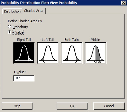
Example 3-11: Probability 'between'
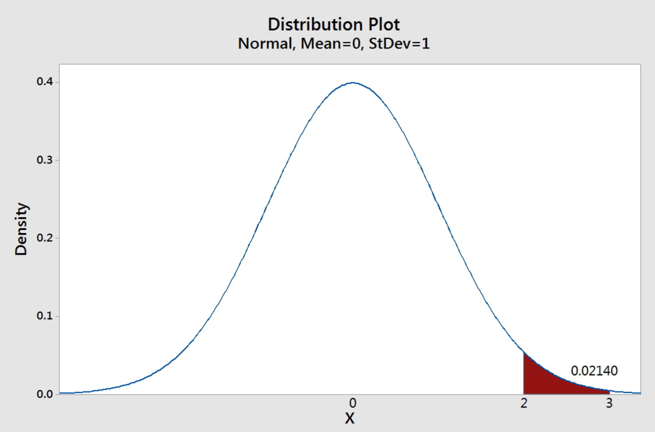
Find the area under the standard normal curve between 2 and 3.
To find the probability between these two values, subtract the probability of less than 2 from the probability of less than 3. In other words,
\(P(2<Z<3)=P(Z<3)-P(Z<2)\)
\(P(Z<3)\) and \(P(Z<2)\) can be found in the table by looking up 2.0 and 3.0.
For 3.0...
z | .00 | .01 | .02 | .03 | .04 | .05 | .06 | .07 | .08 | .09 |
|---|---|---|---|---|---|---|---|---|---|---|
2.8 | 0.9974 | 0.9975 | 0.9976 | 0.9977 | 0.9977 | 0.9978 | 0.9979 | 0.9979 | 0.9980 | 0.9980 |
2.9 | 0.9981 | 0.9982 | 0.9982 | 0.9983 | 0.9984 | 0.9984 | 0.9985 | 0.9985 | 0.9986 | 0.9986 |
3.0 | 0.9987 | 0.9987 | 0.9987 | 0.9988 | 0.9988 | 0.9989 | 0.9989 | 0.9989 | 0.9990 | 0.9990 |
3.1 | 0.9990 | 0.9991 | 0.9991 | 0.9991 | 0.9992 | 0.9992 | 0.9992 | 0.9992 | 0.9993 | 0.9993 |
For 2.0...
z | .00 | .01 | .02 | .03 | .04 | .05 | .06 | .07 | .08 | .09 |
|---|---|---|---|---|---|---|---|---|---|---|
1.8 | 0.9641 | 0.9649 | 0.9656 | 0.9664 | 0.9671 | 0.9678 | 0.9686 | 0.9693 | 0.9699 | 0.9706 |
1.9 | 0.9713 | 0.9719 | 0.9726 | 0.9732 | 0.9738 | 0.9744 | 0.9750 | 0.9756 | 0.9761 | 0.9767 |
2.0 | 0.9772 | 0.9778 | 0.9783 | 0.9788 | 0.9793 | 0.9798 | 0.9803 | 0.9808 | 0.9812 | 0.9817 |
2.1 | 0.9821 | 0.9826 | 0.9830 | 0.9834 | 0.9838 | 0.9842 | 0.9846 | 0.9850 | 0.9854 | 0.9857 |
\(P(2 < Z < 3)= P(Z < 3) - P(Z \le 2)= 0.9987 - 0.9772= 0.0215\).
Using Minitab
To find the area between 2.0 and 3.0 we can use the calculation method in the previous examples to find the cumulative probabilities for 2.0 and 3.0 and then subtract.
\(P(2 < Z < 3)= P(Z < 3) - P(Z \le 2)= 0.9987 - 0.9772= 0.0215\)
You can also use the probability distribution plots in Minitab to find the "between."
- Select Graph> Probability Distribution Plot> View Probability and click OK.
- In the pop-up window select the Normal distribution with a mean of 0.0 and a standard deviation of 1.0.
- Select the Shaded Area tab at the top of the window.
- Select X Value.
- Select Middle.
- Enter 2.0 for X value 1 and 3.0 for X value 2.
- Click OK.
Percentiles of the Standard Normal Distribution
Recall from Lesson 1 that the \(p(100\%)^{th}\) percentile is the value that is greater than \(p(100\%)\) of the values in a data set. We can use the standard normal table and software to find percentiles for the standard normal distribution.
The intersection of the columns and rows in the table gives the probability. If we look for a particular probability in the table, we could then find its corresponding Z value.
Example 3-12: Percentiles in the Standard Normal Distribution
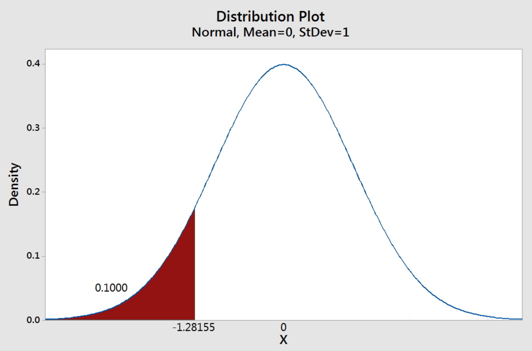
Find the 10th percentile of the standard normal curve.
The question is asking for a value to the left of which has an area of 0.1 under the standard normal curve.
Since the entries in the Standard Normal Cumulative Probability Table represent the probabilities and they are four-decimal-place numbers, we shall write 0.1 as 0.1000 to remind ourselves that it corresponds to the inside entry of the table. We search the body of the tables and find that the closest value to 0.1000 is 0.1003. We look to the leftmost of the row and up to the top of the column to find the corresponding z-value.
The corresponding z-value is -1.28. Thus z = -1.28.
z | .00 | .01 | .02 | .03 | .04 | .05 | .06 | .07 | .08 | .09 |
|---|---|---|---|---|---|---|---|---|---|---|
-1.3 | 0.0968 | 0.0951 | 0.934 | 0.0918 | 0.0901 | 0.0885 | 0.0869 | 0.0853 | 0.0838 | 0.0823 |
-1.2 | 0.1150 | 0.1131 | 0.1112 | 0.1093 | 0.1075 | 0.1056 | 0.1038 | 0.1020 | 0.1003 | 00985 |
-1.1 | 0.1357 | 0.1335 | 0.1314 | 0.1292 | 0.1271 | 0.1251 | 0.1230 | 0.1210 | 0.1190 | 0.1170 |
-1.0 | 0.1587 | 0.1562 | 0.1539 | 0.1515 | 0.1492 | 0.1469 | 0.1446 | 0.1423 | 0.1401 | 0.1379 |
Therefore, the 10th percentile of the standard normal distribution is -1.28.
Using Minitab
To find the 10th percentile of the standard normal distribution in Minitab...
- Select Calc> Probability Distributions> Normal.
- In the new window choose Inverse Cumulative Probability.
- Enter 0.1 in the Input constant box.
- Click OK.
You should see a value very close to -1.28.
Minitab® – Normal Distribution with Minitab
Consider an alternative approach to calculate cumulative probabilities and normal percentiles in Minitab. Additionally, find the instructions for the same computations using the standard normal table for comparison.
Cumulative Probability
Suppose X has a Normal distribution with mean=10 and variance=4, and we want to find a Cumulative Probability: For example, find \(P(X≤12)\):
\(P(X≤12)=P(Z≤\dfrac{12-10}{\sqrt{4}})=P(Z≤1)=0.8413\)
Minitab Method 1 [Graph]:
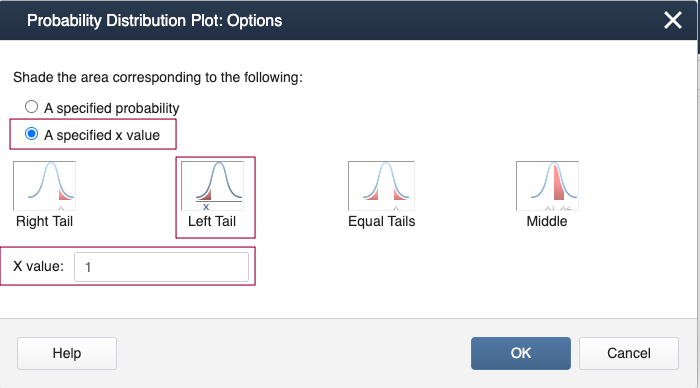
- Select Graph > Probability Distribution Plot>View Probability > Normal (set the mean = 0 and variance = 1).
- In Options, select 'A specified value', 'Left Tail', and X-value: 1
- Select OKand OK
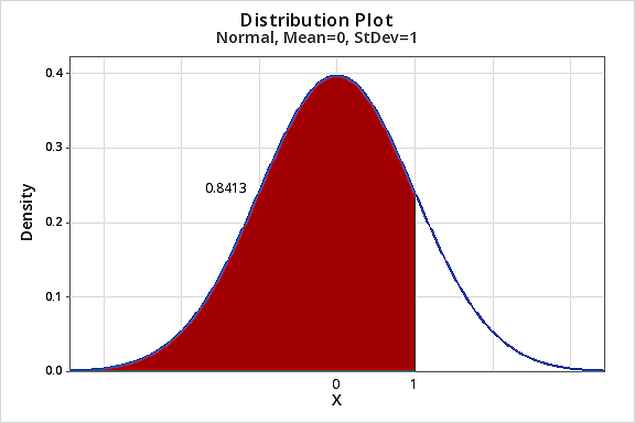
Minitab Method 2 [Calc]:
- Select Calc > Probability Distributions>Cumulative Distribution Function...
- Select 'A single value', Value = 1, Distribution = Normal, Mean = 0 and Standard deviation = 1.
- Select OK
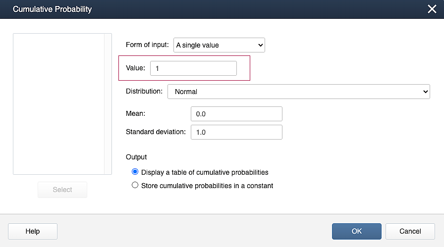
Binomial with n= 3 and p = 0.2
|
x |
P(X≤x) |
|---|---|
|
1 |
0.841345 |
You can read the z-score from the table only to two decimal places. Read up to 1st decimal in the 1st column and the second decimal from the corresponding column as shown below.
|
z |
.00 |
.01 |
.02 |
.03 |
.04 |
.05 |
.06 |
|---|---|---|---|---|---|---|---|
|
0.6 |
.7257 |
.7291 |
.7324 |
.7357 |
.7389 |
.7422 |
.7454 |
|
0.7 |
.7580 |
.7611 |
.7642 |
.7673 |
.7704 |
.7734 |
.7764 |
|
0.8 |
.7881 |
.7910 |
.7939 |
.7967 |
.7995 |
.8023 |
.8051 |
|
0.9 |
.8159 |
.8186 |
.8212 |
.8238 |
.8264 |
.8289 |
.8315 |
|
1.0 |
.8413 |
.8438 |
.8461 |
.8485 |
.8508 |
.8531 |
.8554 |
Therefore, the probability below a Z score of 1 is 0.8413.
Inverse Cumulative Probability
For example, say we want to find the 10th percentile of a normal distribution with a mean = 10 and a variance = 4.
Step 1:
Find the 10th percentile for a standard normal distribution.
That is \(z^*\) find such that \(P(Z≤z^*)=0.10\)→\(z^*=-1.282\)
Minitab Method 1 [Graph]:
- Select Graph > Probability Distribution Plot>View Probability > Normal (set the mean = 0 and variance = 1).
- In Options, select 'A specified value', 'Left Tail', and X-value: 1
- Select OK and OK
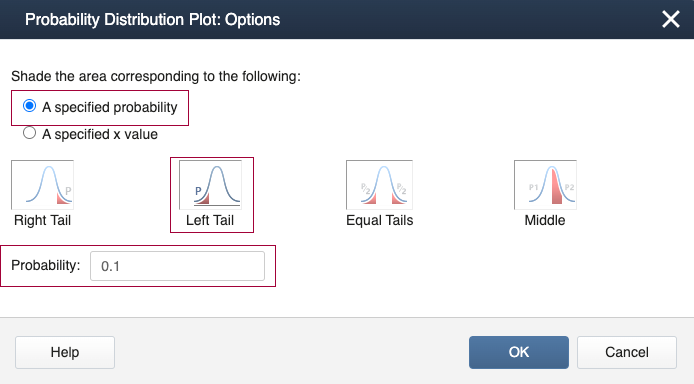
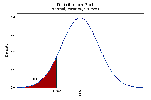
Minitab Method 2 [Calc]:
- Select Calc > Probability Distributions> Inverse Cumulative Distribution Function...
- Select 'A single value', Value = 1, Distribution = Normal, Mean = 0 and Standard deviation = 1.
- Select OK

Normal with mean = 0 and standard deviation = 1
|
x |
P(X≤x) |
|---|---|
|
0.1 |
-1.28155 |
Remember inside the table you have cumulative probabilities. So, you have to look for 0.1 cumulative probability in the table. Since the exact value is not in the table you read the closest value which is 0.1003. Now go to the margins to read the relevant z-score as shown below.
|
z |
.00 |
.01 |
.02 |
.03 |
.04 |
.05 |
.06 |
.07 |
.08 |
.09 |
|---|---|---|---|---|---|---|---|---|---|---|
|
-1.3 |
0.0968 |
0.0951 |
0.934 |
0.0918 |
0.0901 |
0.0885 |
0.0869 |
0.0853 |
0.0838 |
0.0823 |
|
-1.2 |
0.1150 |
0.1131 |
0.1112 |
0.1093 |
0.1075 |
0.1056 |
0.1038 |
0.1020 |
0.1003 |
00985 |
|
-1.1 |
0.1357 |
0.1335 |
0.1314 |
0.1292 |
0.1271 |
0.1251 |
0.1230 |
0.1210 |
0.1190 |
0.1170 |
|
-1.0 |
0.1587 |
0.1562 |
0.1539 |
0.1515 |
0.1492 |
0.1469 |
0.1446 |
0.1423 |
0.1401 |
0.1379 |
Step 2:
Back transform to the original scale.
Now that we have the z-score back transform as below:
\(x^*=10-1.28×2=10-2.56=7.44\)
3.3.3 - Probabilities for Normal Random Variables (Z-scores)
3.3.3 - Probabilities for Normal Random Variables (Z-scores)The standard normal is important because we can use it to find probabilities for a normal random variable with any mean and any standard deviation.
But first, we need to explain Z-scores.
Z-value, Z-score, or Z
We can convert any normal distribution into the standard normal distribution in order to find probability and apply the properties of the standard normal. In order to do this, we use the z-value.
- Z-value, Z-score, or Z
-
The Z-value (or sometimes referred to as Z-score or simply Z) represents the number of standard deviations an observation is from the mean for a set of data. To find the z-score for a particular observation we apply the following formula:
-
\(Z = \dfrac{(observed\ value\ - mean)}{SD}\)
-
Let's take a look at the idea of a z-score within context.
For a recent final exam in STAT 500, the mean was 68.55 with a standard deviation of 15.45.
- If you scored an 80%: \(Z = \dfrac{(80 - 68.55)}{15.45} = 0.74\), which means your score of 80 was 0.74 SD above the mean.
- If you scored a 60%: \(Z = \dfrac{(60 - 68.55)}{15.45} = -0.55\), which means your score of 60 was 0.55 SD below the mean.
Is it always good to have a positive Z score? It depends on the question. For exams, you would want a positive Z-score (indicates you scored higher than the mean). However, if one was analyzing days of missed work then a negative Z-score would be more appealing as it would indicate the person missed less than the mean number of days.
- The scores can be positive or negative.
- For data that is symmetric (i.e. bell-shaped) or nearly symmetric, a common application of Z-scores for identifying potential outliers is for any Z-scores that are beyond ± 3.
- Maximum possible Z-score for a set of data is \(\dfrac{(n−1)}{\sqrt{n}}\)
From Z-score to Probability
For any normal random variable, if you find the Z-score for a value (i.e standardize the value), the random variable is transformed into a standard normal and you can find probabilities using the standard normal table.
For instance, assume U.S. adult heights and weights are both normally distributed. Clearly, they would have different means and standard deviations. However, if you knew these means and standard deviations, you could find your z-score for your weight and height.
You can now use the Standard Normal Table to find the probability, say, of a randomly selected U.S. adult weighing less than you or taller than you.
Example 3-13: Heights
According to the Center for Disease Control, heights for U.S. adult females and males are approximately normal.
- Females: mean of 64 inches and SD of 2 inches
- Males: mean of 69 inches and SD of 3 inches
Find the probability of a randomly selected U.S. adult female being shorter than 65 inches.
Answer
This is asking us to find \(P(X < 65)\). Using the formula \(z=\dfrac{x-\mu}{\sigma}\) we find that:
\(z=\dfrac{65-64}{2}=0.5\)
Now, we have transformed \(P(X < 65)\) to \(P(Z < 0.50)\), where \(Z\) is a standard normal. From the table we see that \(P(Z < 0.50) = 0.6915\). So, roughly there this a 69% chance that a randomly selected U.S. adult female would be shorter than 65 inches.
Example 3-14: Weights
The weights of 10-year-old girls are known to be normally distributed with a mean of 70 pounds and a standard deviation of 13 pounds. Find the percentage of 10-year-old girls with weights between 60 and 90 pounds.
In other words, we want to find \(P(60 < X < 90)\), where \(X\) has a normal distribution with mean 70 and standard deviation 13.
Answer
It is often helpful to draw a sketch of the normal curve and shade in the region of interest. You can either sketch it by hand or use a graphing tool.
To find the probability, we need to first find the Z-scores: \(z=\dfrac{x-\mu}{\sigma}\)
For \(x=60\), we get \(z=\dfrac{60-70}{13}=-0.77\)
For \(x=90\), we get \(z=\dfrac{90-70}{13}=1.54\)
\begin{align*}
P(60<X<90) &= P(-0.77<Z<1.54) &&\text{(Subbing in the Z values from above)} \\
&= P(Z<1.54) - P(Z<-0.77) &&\text{(Subtract the cumulative probabilities)}\\
&=0.9382-0.2206 &&\text{(Use a table or technology)}\\ &=0.7176 \end{align*}
We obtain that 71.76% of 10-year-old girls have weight between 60 pounds and 90 pounds.
Example 3-15: Weights Cont'd...
Find the 60th percentile for the weight of 10-year-old girls given that the weight is normally distributed with a mean 70 pounds and a standard deviation of 13 pounds.
Answer
As before, it is helpful to draw a sketch of the normal curve and shade in the region of interest. You can either sketch it by hand or use a graphing tool. You know that 60% will greater than half of the entire curve.
We can use the Standard Normal Cumulative Probability Table to find the z-scores given the probability as we did before.
Area to the left of z-scores = 0.6000.
The closest value in the table is 0.5987.
The z-score corresponding to 0.5987 is 0.25.
Thus, the 60th percentile is z = 0.25.
Now that we found the z-score, we can use the formula to find the value of \(x\). The Z-score formula is \(z=\dfrac{x-\mu}{\sigma}\).
Using algebra, we can solve for \(x\).
\(x=\mu+z(\sigma)\)
\(x=70+(0.25)(13)=73.25\)
Therefore, the 60th percentile of 10-year-old girls' weight is 73.25 pounds.
3.3.4 - The Empirical Rule
3.3.4 - The Empirical RuleThe Empirical Rule is sometimes referred to as the 68-95-99.7% Rule. The rule is a statement about normal or bell-shaped distributions.
- Empirical Rule
-
In any normal or bell-shaped distribution, roughly...
- 68% of the observations lie within one standard deviation to either side of the mean.
- 95% of the observations lie within two standard deviations to either side of the mean.
- 99.7% of the observations lie within three standard deviations to either side of the mean.
The normal curve showing the empirical rule.
Try It!
Use the normal table to validate the empirical rule. In other words, find the exact probabilities \(P(-1<Z<1)\), \(P(-2<Z<2)\), and \(P(-3<Z<3)\) using the normal table and compare the values to those from the empirical rule.
\(P(-1<Z<1)= P(Z<1)-P(Z<-1) = .8413 - .1587 \approx .68\)
\(P(-2<Z<2)= P(Z<2)-P(Z<-2) = .9772 - .0228 \approx .95\)
\(P(-3<Z<3)= P(Z<3)-P(Z<-3) = .9987 - .0013 \approx .99.7\)
3.3.5 - Other Continuous Distributions
3.3.5 - Other Continuous DistributionsAlthough the normal distribution is important, there are other important distributions of continuous random variables. Some we will introduce throughout the course, but there are many others not discussed. Here are a few distributions that we will see in more detail later.
The t-distribution is a bell-shaped distribution, similar to the normal distribution, but with heavier tails. It is symmetric and centered around zero. The distribution changes based on a parameter called the degrees of freedom. We will discuss degrees of freedom in more detail later.
The graph shows the t-distribution with various degrees of freedom. The standard normal distribution is also shown to give you an idea of how the t-distribution compares to the normal. As you can see, the higher the degrees of freedom, the closer the t-distribution is to the standard normal distribution.
The chi-square distribution is a right-skewed distribution. The distribution depends on the parameter degrees of freedom, similar to the t-distribution. Here is a plot of the Chi-square distribution for various degrees of freedom.
We will see the Chi-square later on in the semester and see how it relates to the Normal distribution.
The F-distribution is a right-skewed distribution. The distribution depends on the two parameters both are referred to as degrees of freedom. The first is typically called the numerator degrees of freedom ($d_1$) and the second is typically referred to as the denominator degrees of freedom ($d_2$). Here is a plot of the F-distribution with various degrees of freedom.
The F-distribution will be discussed in more detail in a future lesson.
3.4 - Lesson 3 Summary
3.4 - Lesson 3 SummaryIn this Lesson, we introduced random variables and probability distributions. There are two main types of random variables, qualitative and quantitative. With the knowledge of distributions, we can find probabilities associated with the random variables.
In the next Lesson, we are going to begin learning how to use these concepts for inference for the population parameters.