4.1 - Sampling Distribution of the Sample Mean

In the following example, we illustrate the sampling distribution for the sample mean for a very small population. The sampling method is done without replacement.

Sample Means with a Small Population: Pumpkin Weights

Image of pumpkins

In this example, the population is the weight of six pumpkins (in pounds) displayed in a carnival "guess the weight" game booth. You are asked to guess the average weight of the six pumpkins by taking a random sample without replacement from the population.

Pumpkin	A	B	C	D	E	F
Weight (in pounds)	19	14	15	9	10	17

Since we know the weights from the population, we can find the population mean.

\(\mu=\dfrac{19+14+15+9+10+17}{6}=14\) pounds

To demonstrate the sampling distribution, let’s start with obtaining all of the possible samples of size \(n=2\) from the populations, sampling without replacement. The table below shows all the possible samples, the weights for the chosen pumpkins, the sample mean and the probability of obtaining each sample. Since we are drawing at random, each sample will have the same probability of being chosen.

Sample	Weight	\(\boldsymbol{\bar{x}}\)	Probability
A, B	19, 14	16.5	\(\frac{1}{15}\)
A, C	19, 15	17.0	\(\frac{1}{15}\)
A, D	19, 9	14.0	\(\frac{1}{15}\)
A, E	19, 10	14.5	\(\frac{1}{15}\)
A, F	19, 17	18.0	\(\frac{1}{15}\)
B, C	14, 15	14.5	\(\frac{1}{15}\)
B, D	14, 9	11.5	\(\frac{1}{15}\)
B, E	14, 10	12.0	\(\frac{1}{15}\)
B, F	14, 17	15.5	\(\frac{1}{15}\)
C, D	15, 9	12.0	\(\frac{1}{15}\)
C, E	15, 10	12.5	\(\frac{1}{15}\)
C, F	15, 17	16.0	\(\frac{1}{15}\)
D, E	9, 10	9.5	\(\frac{1}{15}\)
D, F	9, 17	13.0	\(\frac{1}{15}\)
E, F	10, 17	13.5	\(\frac{1}{15}\)

We can combine all of the values and create a table of the possible values and their respective probabilities.

\(\boldsymbol{\bar{x}}\)	9.5	11.5	12.0	12.5	13.0	13.5	14.0	14.5	15.5	16.0	16.5	17.0	18.0
Probability	\(\frac{1}{15}\)	\(\frac{1}{15}\)	\(\frac{2}{15}\)	\(\frac{1}{15}\)	\(\frac{1}{15}\)	\(\frac{1}{15}\)	\(\frac{1}{15}\)	\(\frac{2}{15}\)	\(\frac{1}{15}\)	\(\frac{1}{15}\)	\(\frac{1}{15}\)	\(\frac{1}{15}\)	\(\frac{1}{15}\)

The table is the probability table for the sample mean and it is the sampling distribution of the sample mean weights of the pumpkins when the sample size is 2. It is also worth noting that the sum of all the probabilities equals 1. It might be helpful to graph these values.

Sampling Distribution

One can see that the chance that the sample mean is exactly the population mean is only 1 in 15, very small. (In some other examples, it may happen that the sample mean can never be the same value as the population mean.) When using the sample mean to estimate the population mean, some possible error will be involved since the sample mean is random.

Now that we have the sampling distribution of the sample mean, we can calculate the mean of all the sample means. In other words, we can find the mean (or expected value) of all the possible \(\bar{x}\)’s.

The mean of the sample means is

\(\mu_\bar{x}=\sum \bar{x}_{i}f(\bar{x}_i)=9.5\left(\frac{1}{15}\right)+11.5\left(\frac{1}{15}\right)+12\left(\frac{2}{15}\right)\\+12.5\left(\frac{1}{15}\right)+13\left(\frac{1}{15}\right)+13.5\left(\frac{1}{15}\right)+14\left(\frac{1}{15}\right)\\+14.5\left(\frac{2}{15}\right)+15.5\left(\frac{1}{15}\right)+16\left(\frac{1}{15}\right)+16.5\left(\frac{1}{15}\right)\\+17\left(\frac{1}{15}\right)+18\left(\frac{1}{15}\right)=14\)

Even though each sample may give you an answer involving some error, the expected value is right at the target: exactly the population mean. In other words, if one does the experiment over and over again, the overall average of the sample mean is exactly the population mean.

Now, let's do the same thing as above but with sample size \(n=5\)

Sample	Weights	\(\boldsymbol{\bar{x}}\)	Probability
A, B, C, D, E	19, 14, 15, 9, 10	13.4	1/6
A, B, C, D, F	19, 14, 15, 9, 17	14.8	1/6
A, B, C, E, F	19, 14, 15, 10, 17	15.0	1/6
A, B, D, E, F	19, 14, 9, 10, 17	13.8	1/6
A, C, D, E, F	19, 15, 9, 10, 17	14.0	1/6
B, C, D, E, F	14, 15, 9, 10, 17	13.0	1/6

The sampling distribution is:

\(\boldsymbol{\bar{x}}\)	13.0	13.4	13.8	14.0	14.8	15.0
Probability	1/6	1/6	1/6	1/6	1/6	1/6

The mean of the sample means is...

\(\mu=(\dfrac{1}{6})(13+13.4+13.8+14.0+14.8+15.0)=14\) pounds

The following dot plots show the distribution of the sample means corresponding to sample sizes of \(n=2\) and of \(n=5\).

Population Mean

Again, we see that using the sample mean to estimate population mean involves sampling error. However, the error with a sample of size \(n=5\) is on the average smaller than with a sample of size \(n= 2\).

Sampling Error and Size

Sampling Error: The error resulting from using a sample characteristic to estimate a population characteristic.

Sample size and sampling error: As the dotplots above show, the possible sample means cluster more closely around the population mean as the sample size increases. Thus, the possible sampling error decreases as sample size increases.

What happens when the population is not small, as in the pumpkin example?

Sample Means with Large Samples: Exam Example

An instructor of an introduction to statistics course has 200 students. The scores out of 100 points are shown in the histogram.

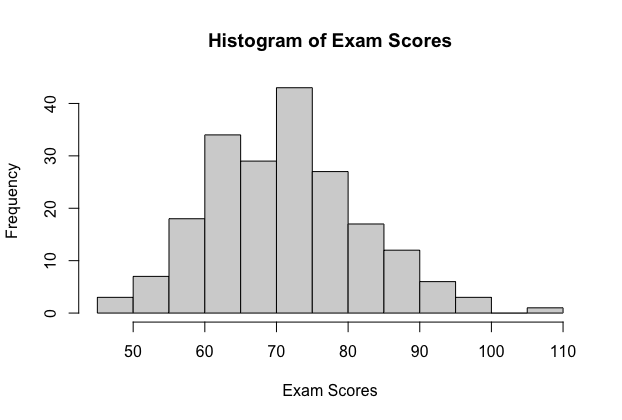
The population mean is \(μ=71.18\) and the population standard deviation is \(σ=10.73\)

Let's demonstrate the sampling distribution of the sample means using the StatKey website. The first video will demonstrate the sampling distribution of the sample mean when n = 10 for the exam scores data. The second video will show the same data but with samples of n = 30.

n=10
n=30

You should start to see some patterns. The mean of the sampling distribution is very close to the population mean. The standard deviation of the sampling distribution is smaller than the standard deviation of the population.

In the examples so far, we were given the population and sampled from that population.

What happens when we do not have the population to sample from? What happens when all that we are given is the sample? Fortunately, we can use some theory to help us. The mathematical details of the theory are beyond the scope of this course but the results are presented in this lesson.

In the next two sections, we will discuss the sampling distribution of the sample mean when the population is Normally distributed and when it is not.

4.1.1 - Population is Normal

If the population is normally distributed with mean \(\mu\) and standard deviation \(\sigma\), then the sampling distribution of the sample mean is also normally distributed no matter what the sample size is. When the sampling is done with replacement or if the population size is large compared to the sample size, then \(\bar{x}\) has mean \(\mu\) and standard deviation \(\dfrac{\sigma}{\sqrt{n}}\). We use the term standard error for the standard deviation of a statistic, and since sample average, \(\bar{x}\) is a statistic, standard deviation of \(\bar{x}\) is also called standard error of \(\bar{x}\). However, in some books you may find the term standard error for the estimated standard deviation of \(\bar{x}\). In this class we use the former definition, that is, standard error of \(\bar{x}\) is the same as standard deviation of \(\bar{x}\).

Standard Deviation of \(\boldsymbol{\bar{x}}\) [Standard Error]: \(SD(\bar{X})=SE(\bar{X})=\dfrac{\sigma}{\sqrt{n}}\)

When we know the sample mean is Normal or approximately Normal, then we can calculate a z-score for the sample mean and determine probabilities for it using:

Z-Score of the Sample Mean: \(z=\dfrac{\bar{x}-\mu}{\dfrac{\sigma}{\sqrt{n}}}\)

Example 4-1: Speedboat Engines

The engines made by Ford for speedboats have an average power of 220 horsepower (HP) and standard deviation of 15 HP. You can assume the distribution of power follows a normal distribution.

Consumer Reports® is testing the engines and will dispute the company's claim if the sample mean is less than 215 HP. If they take a sample of 4 engines, what is the probability the mean is less than 215?

Answer

We want to find \(P(\bar{X}<215)\).

Since the population follows a normal distribution, we can conclude that \(\bar{X}\) has a normal distribution with mean 220 HP (\(\mu=220\)) and a standard deviation of \(\dfrac{\sigma}{\sqrt{n}}=\dfrac{15}{\sqrt{4}}=7.5\)HP.

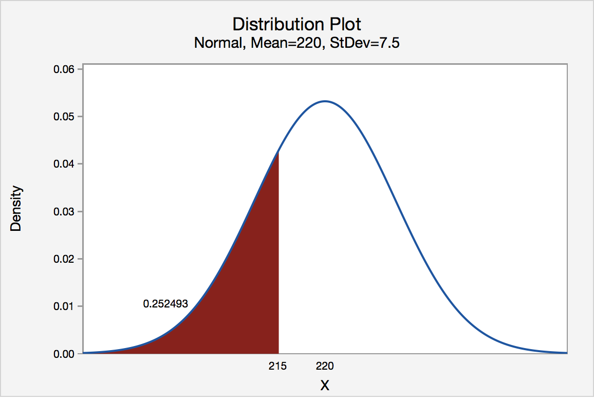
Normal distribution probability plot of area below 215.

\(P(\bar{X}<215)=P\left(Z<\dfrac{215-220}{7.5}\right)=P(Z<-0.67) \approx\ 0.2514\)

If Consumer Reports® samples four engines, the probability that the mean is less than 215 HP is 25.14%.

Try It!

Using the speedboat engines example above, answer the following question.

If Consumer Reports® samples 100 engines, what is the probability that the sample mean will be less than 215?

The sampling distribution of the sample mean is Normal with mean \(\mu=220\) and standard deviation \(\dfrac{\sigma}{\sqrt{n}}=\dfrac{15}{\sqrt{100}}=1.5\).

\(P(\bar{X}<215)=P\left(\dfrac{\bar{X}-\mu}{\dfrac{\sigma}{\sqrt{n}}}<\dfrac{215-220}{1.5}\right)=P\left(Z<-\dfrac{10}{3}\right)=0.00043\).

It is worth noting the difference in the probabilities here. When the sample size is \(n=4\), the probability of obtaining a sample mean of 215 or less is 25.14%. When the sample size is \(n=100\), the probability is 0.043%.

4.1.2 - Population is Not Normal

Central Limit Theorem

What happens when the sample comes from a population that is not normally distributed? This is where the Central Limit Theorem comes in.

Central Limit Theorem

For a large sample size (we will explain this later), \(\bar{x}\) is approximately normally distributed, regardless of the distribution of the population one samples from. If the population has mean \(\mu\) and standard deviation \(\sigma\), then \(\bar{x}\) has mean \(\mu\) and standard deviation \(\dfrac{\sigma}{\sqrt{n}}\).

We should stop here to break down what this theorem is saying because the Central Limit Theorem is very powerful!

The Central Limit Theorem applies to a sample mean from any distribution. We could have a left-skewed or a right-skewed distribution. As long as the sample size is large, the distribution of the sample means will follow an approximate Normal distribution.

For the purposes of this course, a sample size of \(n>30\) is considered a large sample.

CLT Demonstration

Before we begin the demonstration, let's talk about what we should be looking for…

Notes on the CLT for this demonstration:

If the population is skewed and sample size small, then the sample mean won't be normal.
When doing a simulation, one replicates the process many times. Using 10,000 replications is a good idea.
If the population is normal, then the distribution of sample mean looks normal even if \(n = 2\). Note the app in the video used capital N for the sample size.
If the population is skewed, then the distribution of sample mean looks more and more normal when \(n\) gets larger.
Note that in all cases, the mean of the sample mean is close to the population mean and the standard error of the sample mean is close to \(\dfrac{\sigma}{\sqrt{n}}\).

To work through this demonstration of the central limit theorem yourself, click on the link to the website, Rice Virtual Lab in Statistics > Sampling Distributions, and then click Begin.

Sampling Distribution of the Sample Mean

With the Central Limit Theorem, we can finally define the sampling distribution of the sample mean.

Sampling Distribution of the Sample Mean

The sampling distribution of the sample mean will have:

The same mean as the population mean, \(\mu\).
Standard deviation [standard error] of \(\dfrac{\sigma}{\sqrt{n}}\).

It will be Normal (or approximately Normal) if either of these conditions is satisfied:

The population distribution is Normal.
The sample size is large (\(n \gt 30\)).

Example 4-2: Weights of Baby Giraffes

Giraffes in a field

The weights of baby giraffes are known to have a mean of 125 pounds and a standard deviation of 15 pounds.

If we obtained a random sample of 40 baby giraffes,

what is the probability that the sample mean will be between 120 and 130 pounds?
what is the 75th percentile of the sample means of size \(n=40\)?

Answer

Does the problem indicate that the distribution of weights is normal? No, it does not. In order to apply the Central Limit Theorem, we need a large sample. Since \(n=40>30\), we can use the theorem. The sampling distribution of the sample mean is approximately Normal with mean \(\mu=125\) and standard error \(\dfrac{\sigma}{\sqrt{n}}=\dfrac{15}{\sqrt{40}}\).

We want \(P(120<\bar{X}<130)\).
\begin{align} P(120<\bar{X}<130) &=P\left(\dfrac{120-125}{\dfrac{15}{\sqrt{40}}}<\dfrac{\bar{X}-\mu}{\dfrac{\sigma}{\sqrt{n}}}<\frac{130-125}{\dfrac{15}{\sqrt{40}}}\right)\\ &=P(-2.108<Z<2.108)\\&=P(Z<2.108)-P(Z<-2.108)\\ &=0.9826-0.0174\\ &=0.9652 \end{align}

The probability that the sample mean of the 40 giraffes is between 120 and 130 lbs is 96.52%.
To find the 75th percentile, we need the value \(a\) such that \(P(Z<a)=0.75\). Using the Z-table or software, we get \(a=.6745\). The formula for the z-score is...

\(z=\dfrac{\bar{X}-\mu}{\dfrac{\sigma}{\sqrt{40}}}=\dfrac{\bar{X}-125}{\dfrac{15}{\sqrt{40}}}\)

Since we know the \(z\) value is 0.6745, we can use algebra to solve for \(\bar{X}\).

\begin{align} 0.6745&=\dfrac{\bar{X}-125}{\frac{15}{\sqrt{40}}}\\
0.6745\left(\frac{15}{\sqrt{40}}\right) &=\bar{X}-125\\
\bar{X}&=0.6745\left(\frac{15}{\sqrt{40}}\right)+125\\&=126.6 \end{align}

The 75th percentile of all the sample means of size \(n=40\) is \(126.6\) pounds.

^[1]	Link
↥	Has Tooltip/Popover
	Toggleable Visibility