5.3 - Inference for the Population Proportion
5.3 - Inference for the Population ProportionEarlier in the lesson, we talked about two types of estimation, point, and interval. Let's now apply them to estimate a population proportion from sample data.
Point Estimate for the Population Proportion
The point estimate of the population proportion, \(p\), is:
Point Estimate of the Population Proportion
\(\hat{p}=\dfrac{\text{# of successes in the sample}}{\text{sample size, n}}\)
From our previous lesson on sampling distributions, we know the sampling distribution of the sample proportion under certain conditions. We can use this information to construct a confidence interval for the population proportion.
Confidence Interval for the Population Proportion
Recall that:
If \(np\) and \(n(1-p)\) are greater than five, then \(\hat{p}\) is approximately normal with mean, \(p\), standard error \(\sqrt{\frac{p(1-p)}{n}}\).
Under these conditions, the sampling distribution of the sample proportion, \(\hat{p}\), is approximately Normal. The multiplier used in the confidence interval will come from the Standard Normal distribution.
5.3.1 - Construct and Interpret the CI
5.3.1 - Construct and Interpret the CIConstructing a Confidence Interval for the Population Proportion
To construct a confidence interval we're going to use the following 3 steps:
- CHECK CONDITIONS
Check all conditions before using the sampling distribution of the sample proportion.
We previously used \(np\) and \(n(1-p)\). But \(p\) is not known. Therefore, for the confidence interval, we will use
- \(n\hat{p}>5\) and
- \(n(1-\hat{p})>5\)
What can one do if the conditions are NOT satisfied?
For a confidence interval for a proportion, there is a technique called exact methods. These methods can be used if the software offers it. These exact methods are more complicated and are based on the relationship between the binomial and another distribution we will later learn called the F-distribution. The Z-method is much simpler and fairly easy to compute. In fact if you ever come across a published random survey (e.g. a Gallup poll) you can use the methods in this lesson to construct a reliable proportion confidence interval rather quickly. - CONSTRUCT THE GENERAL FORM
The general form of the confidence interval is '\(\text{point estimate }\pm M\times \hat{SE}(\text{estimate})\).' The point estimate is the sample proportion, \(\hat{p}\), and the estimated standard error is \(\hat{SE}(\hat{p})=\sqrt{\frac{\hat{p}(1-\hat{p})}{n}}\). If the conditions are satisfied, then the sampling distribution is approximately normal. Therefore, the multiplier comes from the normal distribution. This interval is also known as the one-sample z-interval for \(p\), or the Normal Approximation confidence interval for \(p\).
- \(\boldsymbol{\left(1-\alpha \right) 100\%}\) confidence interval for the population proportion, \(\boldsymbol{p}\)
- \(\hat{p}\pm z_{\alpha/2}\sqrt{\dfrac{\hat{p}(1-\hat{p})}{n}}\)
- where \(z_{\alpha/2}\) represents a z-value with \(\alpha/2\) area to the right of it.
General notes about the confidence interval...
- The \(\pm\) in the formula above means "plus or minus". It is a shorthand way of writing
\((\hat{p}-z_{\alpha/2}\sqrt{\frac{\hat{p}(1-\hat{p})}{n}}, \hat{p}+z_{\alpha/2}\sqrt{\frac{\hat{p}(1-\hat{p})}{n}})\)
- It is centered at the point estimate, \(\hat{p}\).
- The width of the interval is determined by the margin of error.
- You must determine the multiplier.
- INTERPRET THE CONFIDENCE INTERVAL
Applying the template from earlier in the lesson we can say we are \((1-\alpha)100\%\) confident that the population proportion is between \(\hat{p}-z_{\alpha/2}\sqrt{\frac{\hat{p}(1-\hat{p})}{n}}\) and \(\hat{p}+z_{\alpha/2}\sqrt{\frac{\hat{p}(1-\hat{p})}{n}}\). The examples will go into more detail regarding the interpretation of the confidence interval.
Derivation of the Confidence Interval
To calculate the confidence interval, we need to know how to find the z-multiplier. So where does this \(z_{\alpha}\) come from?
The confidence interval can be derived from the following fact:
\begin{align} P\left(\left|\frac{\hat{p}-p}{\sqrt{\dfrac{\hat{p}(1-\hat{p})}{n}}}\right|\le z_{\alpha/2}\right)=1-\alpha \\ P\left(-z_{\alpha/2}\le \dfrac{\hat{p}-p}{\sqrt{\dfrac{\hat{p}(1-\hat{p})}{n}}}\le z_{\alpha/2}\right)=1-\alpha \\ P\left(\hat{p}-z_{\alpha/2}\sqrt{\dfrac{\hat{p}(1-\hat{p})}{n}}\le p \le \hat{p}+z_{\alpha/2}\sqrt{\dfrac{\hat{p}(1-\hat{p})}{n}}\right)=1-\alpha \end{align}
The figure shows the general confidence interval on the normal curve.
How to find the multiplier using the Standard Normal Distribution
\(z_a\) is the z-value having a tail area of \(a\) to its right. With some calculation, one can use the Standard Normal Cumulative Probability Table to find the value.
Example 5-1: Finding \(\boldsymbol{z_a}\)
Find using the standard Normal table: \(z_{0.15}\)
Answer
\(z_{0.15}\) means \(P(Z>z_{0.15})=0.15\). This implies that \(P(Z\le z_{0.15})=0.85\). The value from the table is 1.04.
For more detailed directions on reading the z-table or using Minitab refer to the examples on this page: 3.3.2 The Standard Normal Distribution.
Try it!
Use the Standard Normal Table to find the following:
Commonly Used Alpha Levels
The table is a list of frequently used alphas and their \(z_{\alpha/2}\) multipliers.
| Confidence Level | \(\boldsymbol{\alpha}\) | \(\boldsymbol{z_{\alpha/2}}\) | \(\boldsymbol{z_{\alpha/2}}\) Multiplier |
|---|---|---|---|
| 90% | .10 | \(z_{0.05}\) | 1.645 |
| 95% | .05 | \(z_{0.025}\) | 1.960 |
| 98% | .02 | \(z_{0.01}\) | 2.326 |
| 99% | .01 | \(z_{0.005}\) | 2.576 |
The value of the multiplier increases as the confidence level increases. This leads to wider intervals for higher confidence levels. We are more confident of catching the population value when we use a wider interval.
Example 5-2: Alpha Levels
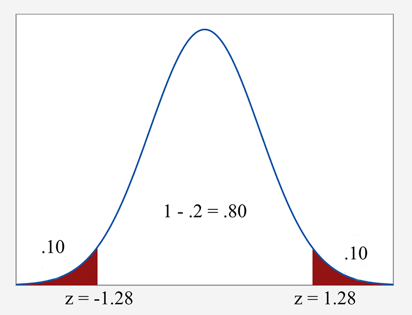
For an 80% confidence interval find \(\alpha\), \(\alpha/2\), and \(z_{\alpha/2}\).
Answer
Recall that \(\alpha\) is used to find the confidence level by taking (1 - \(\alpha)*100%\).
So for an 80% confidence we would take...
\( (1 - \alpha)*100 = 80 \) or...
\((1 - \alpha) = .8\)
\( \alpha = .2\)
Therefore, \(\alpha/2 = .2/2 = .1\)
We would have \(z_{0.10}\) which means \(P(Z>z_{0.10})=0.10\).
This implies that \(P(Z\le z_{0.10})=0.90\). The value from the table is 1.28.
Visually, you can see how these numbers relate to the normal distribution in the graph below.
Example 5-3: Approval Ratings
 A random sample of 1500 U.S. adults is taken. They are asked whether they approve or disapprove of the current president's performance so far (i.e. an approval rating). Of the 1500 surveyed, 660 respond with "approve". Calculate a 95% confidence interval for the overall approval rating of the the president.
Answer
Since we're dealing with a single proportion, we will examine the number of "successes" and the number of "failures". In this example there were 660 successes and 840 failures. With both successes and failures being at least 5, the condition to use the z-method to calculate the interval is acceptable.
For 95% confidence, the alpha value is 5% or 0.05 The multiplier would be a z-value with \(\alpha/2\), or 0.025 area to the right of it. Examining the standard normal table, we find that this corresponds to a z-value of 1.96.
Important Note: Many students tend to use the multiplier of 2 instead of 1.96 due to the empirical rule. As a general rule, it is always best to use the exact values rather than the rounded value.
In this example, we have a sample proportion, \(\hat{p}\), of 660/1500 = 0.44 and a sample size, \(n\), of 1500.\begin{align} \hat{p}& \pm z_{\alpha/2}\sqrt{\dfrac{\hat{p}(1-\hat{p}}{n}} &&\text{(General Form)} \\0.44 &\pm 1.96 \sqrt{\dfrac{0.44(1-0.44)}{1500}} &&\text{(Plug in the numbers)} \\ 0.44 &\pm 0.025 &&\text{(Simplify)}\end{align}
"We are 95% confident that the overall U.S. adult approval rating for the current president is from 41.5% to 46.5%." You could also see this written as, "The current U.S. approval rating for the president is 44% with a 95% margin of error of 2.5%." Commonly, the standard level of confidence is 95% so that reference is often left out as that is the assumed level of confidence unless otherwise stated. Also, the method calculates a proportion but often the reported values are converted to percentages. If you use the decimal formal (e.g. 0.415 and 0.465) then reference these as proportion and not percentage.
View the video explanation from Dr. Bulathsinhala
- In Minitab choose Stat > Basic Statistics > 1 proportion .
- From the drop down box select the Summarized data option button. (If you have the raw data you would use the default drop down of One or more samples, each in a column.)
- Enter the number of successes in the Number of Events text box, and the sample size in the Number of Trials text box.
- Choose the Options button. The default confidence level is 95. If your desire another confidence level edit appropriately.
- To use the z- interval method choose Normal Approximation from the Method text box. The exact interval is always appropriate and is the default. Under the conditions that: $n \hat{p} \ge 5, n(1− \hat{p}) \ge 5$, one can also use the z-interval to approximate the answers. The exact interval and the z-interval should be very similar when the conditions are satisfied.
- Choose OK and OK again.
Using Minitab: Approval Ratings Example
We will now use Minitab to verify our by-hand results. Recall in that example a random sample of 1500 was taken from the population of U.S. adults, with 660 responding with a positive approval.
Answer
In Minitab and following the steps above, we would enter 660 for the Number of Events and 1500 for the Number of Trials. The confidence level was 95% and we satisfied the necessary conditions to use the Normal Approximation (or z-interval) method. The results are:
Test and CI for One Proportion
| Sample | X | N | Sample p | 95% CI |
|---|---|---|---|---|
| 1 | 660 | 1500 | 0.440000 | (0.414880, 0.465120) |
Using the normal approximation.
These results closely match our by-hand interval of 0.415 to 0.465
What if we had calculated the exact confidence interval (i.e. did not choose Normal Approximation as the method)? With the exact method the interval is (0.414685, 0.465550). Consistent to three decimal places in this case. You will notice that in the output Minitab does provide a notification that the normal approximation was used.
We want to know the proportion of graduate students at Penn State who are Democrats. To answer the question, we give out the following survey:
Are you a Democrat? Please circle one answer.
- Yes
- No
Suppose that we get 10 people that circled Yes and 20 people that circled No (that includes the case when people don't know whether they are Democrats!!)
- Let X = the number of successes (number of students who chose Yes) = 10
- n = number of trials = 30
Find a 90% confidence interval for the proportion of graduate students who are democrats.
You should first check the conditions. We know \(\hat{p}=\frac{10}{30}=0.333\) and \(n=30\) Therefore, \(n\hat{p}=30(0.333)=10\) and \(n(1-\hat{p})=20\). Since both values are greater than 5, we can use the Normal distribution.
The z multiplier will be \(z_{0.1/2}=1.645\)
\(\hat{p}\pm 1.645\sqrt{\dfrac{\hat{p}(1-\hat{p})}{n}}=0.333\pm 1.645\sqrt{\dfrac{0.333(1-0.333)}{30}}=0.333\pm0.1415=(0.1915, 0.4745)\).
We are 90% confident that the population proportion of graduate students at Penn State who are democrats is between 19.15% and 47.45%.
The video demonstrates this same example using Minitab.
5.3.2 - Interpreting the CI
5.3.2 - Interpreting the CIMore on the Interpretation of a Confidence Interval
In the graph below, we show 10 replications (for each replication, we sample 30 students and ask them whether they are Democrats) and compute an 80% Confidence Interval each time. We are lucky in this set of 10 replications and get exactly 8 out of 10 intervals that contain the parameter. Due to the small number of replications (only 10), it is quite possible that we get 9 out of 10 or 7 out of 10 that contain the true parameter. On the other hand, if we try it 10,000 (a large number of) times, the percentage that contains the true proportions will be very close to 80%.
If we repeatedly draw random samples of size n from the population where the proportion of success in the population is $p$ and calculate the confidence interval each time, we would expect that $100(1 - \alpha)$% of the intervals would contain the true parameter, $p$.
5.3.3 - Sample Size Computation
5.3.3 - Sample Size ComputationSample Size Computation for the Population Proportion Confidence Interval
An important part of obtaining desired results is to get a large enough sample size. We can use what we know about the margin of error and the desired level of confidence to determine an appropriate sample size.
Recall that the margin of error, E, is half of the width of the confidence interval. Therefore for a one sample proportion,
\(E=z_{\alpha/2}\sqrt{\dfrac{\hat{p}(1-\hat{p})}{n}}\)
- Precision
- The wider the interval, the poorer the precision. Note that the higher the confidence level, the wider the width (or equivalently, half width) of the interval and thus the poorer the precision.
Since the confidence level reflects the success rate of the method we use to get the confidence interval, we like to have a narrower interval while keeping the confidence level at a reasonably higher level.
For most newspapers and magazine polls, it is understood that the margin of error is calculated for a 95% confidence interval (if not stated otherwise). A 3% margin of error is a popular choice also. For instance, you might see a television poll state that the "approval rating of the president is 72%; the margin of error of the poll is plus or minus 3%."
If we want the margin of error smaller (i.e., narrower intervals), we can increase the sample size. Or, if you calculate a 90% confidence interval instead of a 95% confidence interval, the margin of error will also be smaller. However, when one reports it, remember to state that the confidence interval is only 90% because otherwise, people will assume 95% confidence.
Determining the Required Sample Size
If the desired margin of error E is specified and the desired confidence level is specified, the required sample size to meet the requirements can be calculated by two methods:
- Educated Guess
- \(n=\dfrac{z^2_{\alpha/2}\hat{p}_g(1-\hat{p}_g)}{E^2}\)
Where \(\hat{p}_g\) is an educated guess for the parameter \(p\).
*The educated guess method is used if it is relatively inexpensive to sample more elements when needed.
- Conservative Method
- \(n=\dfrac{z^2_{\alpha/2}(\frac{1}{2})^2}{E^2}\)
- This formula can be obtained from part (a) using the fact that:
For \(0 \le p \le 1, p (1 - p)\) achieves its largest value at \(p=\frac{1}{2}\).
*The conservative method is used if the start-up cost of sampling is expensive and thus it is not economical to sample more elements later.
The sample size obtained from using the educated guess is usually smaller than the one obtained using the conservative method. This smaller sample size means there is some risk that the resulting confidence interval may be wider than desired. Using the sample size by the conservative method has no such risk.
Example 5-4
Suppose a television poll states that the "approval rating of the president is 72%." For the next poll of the president's approval rating, we want to get a margin of error of 1% with 95% confidence. How many individuals should we sample?
Answer
Educated Guess:
\(z_{0.025} = 1.96, E = 0.01\)
Therefore,
\(n=\dfrac{(1.96)^2(0.72)(1-0.72)}{(0.01)^2}=7744.67\)
The sample size needed is 7745 people . We always need to round up to the next integer when the result is not a whole number. We discuss this in detail below.
Conservative Method:
\(z_{0.025} = 1.96, E = 0.01\)
Therefore,
\(n=\dfrac{(1.96)^2(0.5)(1-0.5)}{(0.01)^2}=9604\)
The sample size is 9604 people .
Cautions About Sample Size Calculations
- Why do we need to round up?
Because we are estimating the smallest sample size needed to produce the desired error. Since we cannot sample a portion of a subject (e.g. we cannot take 0.66 of a subject) we need to round up to guarantee a large enough sample.
- Remember that this is the minimum sample size needed for our study.
If we encounter a situation where the response rate is not 100% then if we just sample the calculated size, in the end, we will end up with a less than desired sample size. To counter this, we can adjust the calculated sample size by dividing by an anticipated response rate. For instance, using the above example if we expected about 40% of the those contacted to actually participate in our survey (i.e. a 40% response rate) then we would need to sample 7745/0.4=19,362.5 or 19,363. In other words, our actual sample size would need to be 19,363 given the 40% response rate.