5.4 - Inference for the Population Mean

Overview

In this section, we discuss how to find confidence intervals for the population mean. The idea and interpretation of the confidence interval will be similar to that of the population proportion only applied to the population mean, $\mu$.

We start with the case where the population standard deviation, $\sigma$, is known. We continue to the more realistic case where $\sigma$ is not known. For the latter case, we need to recall the $t$-distribution. We end this section by presenting how to determine a sample size for a desired margin of error and confidence.

Point Estimates for a Population Mean

The point estimate of the population mean, $\mu$ is:

Point Estimate of the Population Mean: $\bar{x}=$ sample mean

If one wants to know how accurate the sample mean is to estimate the population mean, we need some probability statement. We will want to know the sampling distribution of $\bar{x}$. From this distribution, we can get a confidence interval. Such an interval provides a range of values for which the parameter value is believed to fall. An interval is more likely to be "correct" than a point estimate.

5.4.1 - Construct and Interpret the CI

Constructing a Confidence Interval for the Population Mean

To construct a confidence interval for a population mean, we're going to apply the same three steps as with the population proportion, but first, let's look at the two possible cases.

Case 1: $\sigma$ is known

In the previous lesson, we learned that if the population is normal with mean $\mu$ and standard deviation, $\sigma$, then the distribution of the sample mean will be Normal with mean $\mu$ and standard error $\frac{\sigma}{\sqrt{n}}$.

Following the similar idea to developing the confidence interval for $p$, the $(1-\alpha)$100% confidence interval for the population mean $\mu$ is...

$P\left(\left|\dfrac{\bar{x}-\mu}{\dfrac{\sigma}{\sqrt{n}}}\right|\le z_{\alpha/2}\right)=1-\alpha$

A little bit of algebra will lead you to...

$P\left(\bar{x}-z_{\alpha/2}\dfrac{\sigma}{\sqrt{n}}\le \mu\le \bar{x}+z_{\alpha/2}\dfrac{\sigma}{\sqrt{n}}\right)=1-\alpha$

In other words, the $(1-\alpha)$100% confidence interval for $\mu$ is:

$\bar{x}\pm z_{\alpha/2}\dfrac{\sigma}{\sqrt{n}}$

Notice for this case, the only condition we need is the population distribution to be normal.

Note!

The case where $\sigma$ is known is unrealistic. We explain it here briefly because it reinforces what we have previously learned. We do not present examples in this case.

Case 2: $\sigma$ is unknown

When the population is normal or when the sample size is large then,

$Z=\dfrac{\bar{x}-\mu}{\dfrac{\sigma}{\sqrt{n}}}$

where Z has a standard Normal distribution.

Usually, we don't know $\sigma$, so what can we do?

Recall that if X comes from a normal distribution with mean, $\mu$, and variance, $\sigma^2$, or if $n\ge 30$, then the sampling distribution will be approximately normal with mean $\mu$ and standard error, $SE(\bar{X})=\frac{\sigma}{\sqrt{n}}$

One way to estimate $\sigma$ is by $s$, the standard deviation of the sample, and replace $\sigma$ by $s$ in the above Z-equation. However, this new quotient no longer has a Z-distribution. Instead it has a t-distribution. We call the following a 'studentized' version of $\bar{X}$:

$t=\dfrac{\bar{X}-\mu}{\dfrac{s}{\sqrt{n}}}$

Constructing the Confidence Interval

CHECK THE CONDITIONS

One of the following conditions need to be satisfied:
1. If the sample comes from a Normal distribution, then the sample mean will also be normal. In this case, $\dfrac{\bar{x}-\mu}{\frac{s}{\sqrt{n}}}$ will follow a $t$-distribution with $n-1$ degrees of freedom.
2. If the sample does not come from a normal distribution but the sample size is large ($n\ge 30$), we can apply the Central Limit Theorem and state that $\bar{X}$ is approximately normal. Therefore, $\dfrac{\bar{x}-\mu}{\frac{s}{\sqrt{n}}}$ will follow a $t$-distribution with $n-1$ degrees of freedom.
CONSTRUCT THE GENERAL FORM

$(1-\alpha)$100% Confidence Interval for the Population Mean, $\mu$

$\bar{x}\pm t_{\alpha/2}\dfrac{s}{\sqrt{n}}$
where the t-distribution has $df = n - 1$. This interval is also known as the one-sample t-interval for the population mean.
INTERPRET THE CONFIDENCE INTERVAL

We are $(1-\alpha)100\%$ confident that the population mean, $\mu$, is between $\bar{x}-t_{\alpha/2}\frac{s}{\sqrt{n}}$ and $\bar{x}+t_{\alpha/2}\frac{s}{\sqrt{n}}$.

What if the conditions are not met?

What will you do if you cannot use the t-interval? What do we do when the above conditions are not satisfied?

If you do not know if the distribution comes from a normally distributed population and the sample size is small (i.e $n<30$), you can use the Normal Probability Plot to check if the data come from a normal distribution.
You may want to consider what is known as nonparametric statistical methods. A procedure such as the one-sample Wilcoxon procedure. Lesson 11 introduces nonparametric statistical methods.

5.4.2 - The t-distribution

In 1908, William Sealy Gosset from Guinness Breweries discovered the t-distribution. His pen-name was Student and thus it is called the "Student's t-distribution."

The t-distribution is different for different sample size, n. Thus, tables, as detailed as the standard normal table, are not provided in the usual statistics books. The graph below shows the t-distribution for degrees of freedom of 10 (blue) and 30 (red dashed).

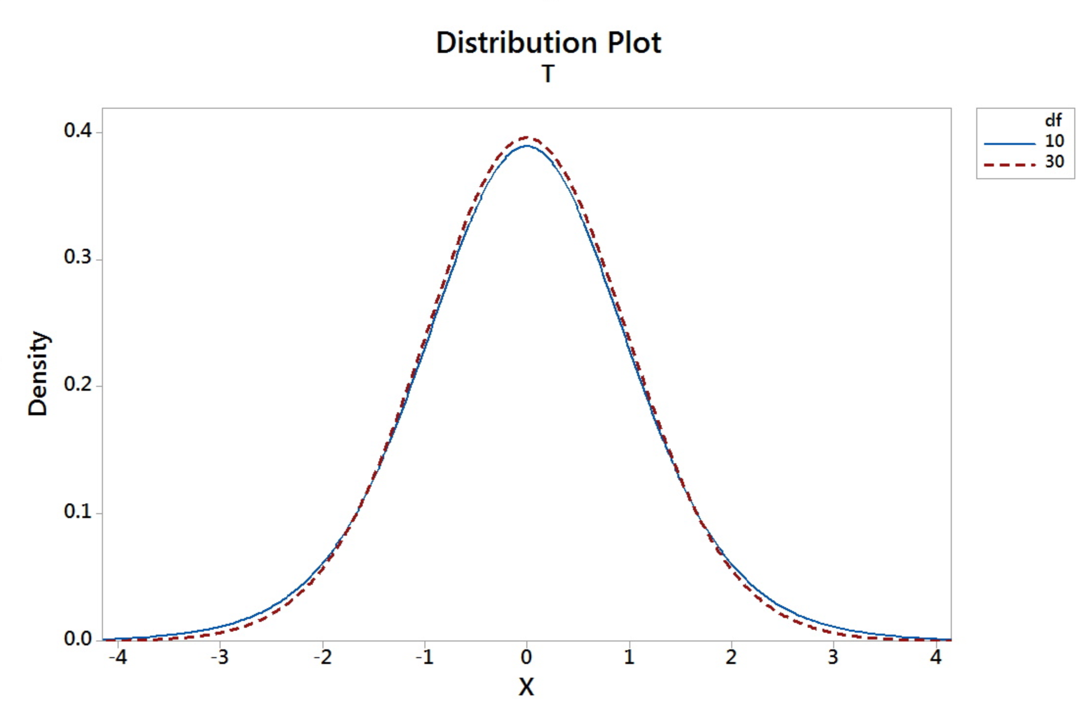
T-distribution graph with degrees freedom fo 10 and 30 — t-distribution

Properties of the t-distribution

t is symmetric about 0
t-distribution is more variable than the Standard Normal distribution
t-distributions are different for different degrees of freedom (d.f.).
The larger $n$ gets (or as $n$ goes to infinity), the closer the $t$-distribution is to the $z$.
The meaning of $t_\alpha$ is the $t$-value having the area "$\alpha$" to the right of it.

Example 5-5: Finding t-values

Use this t-table or the one in your text to find following the example.

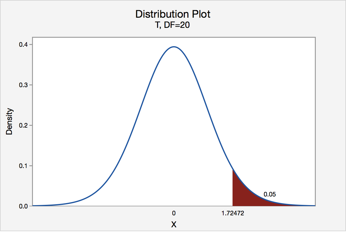
Find $t_{0.05}$ where the degree of freedom is 20.

In a t-distribution table below the top row represents the upper tail area, while the first column are the degrees of freedom.

The $t_{0.05}$ where the degree of freedom is 20 is 1.725 .

df	0.40	0.25	0.10	0.05	0.025	0.01	0.005	0.001	.0005
...	...	...	...	...	...	...	...	...	...
18	0.257	0.688	1.330	1.734	2.101	2.552	2.878	3.610	3.922
19	0.257	0.688	1.328	1.729	2.093	2.539	2.861	3.579	3.883
20	0.257	0.687	1.325	1.725	2.086	2.528	2.845	3.552	3.850
21	0.257	0.686	1.323	1.721	2.080	2.518	2.831	3.527	3.819

The graph shows that the $\alpha$ values at the top of this table are the upper tail areas of the distribution.

t-distribution curve showing a t value of 1.725

Note! When the corresponding degree of freedom is not given in the table, you can use the value for the closest degree of freedom that is smaller than the given one. We use this approach since it is better to err in a conservative manner (get a t-value that is slightly larger than the precise t-value).

Find $t_{0.05}$ where the degree of freedom is 34.

What do we do when the degrees of freedom are not on the table? The t-table degrees of freedom run continuously from 1 to 30, then go by intervals after 30 (e.g. after 30 we have 35). In such cases, we can use software such as Minitab to find a more exact value for the multiplier as opposed to using a degrees of freedom that is "close".

To find the t-value in Minitab...

From the Minitab Menu select Calc > Probability Distributions > t...
Choose inverse cumulative probability
Enter the degrees of freedom
Set the input constant as 0.95 (1 - 0.05).
Choose OK

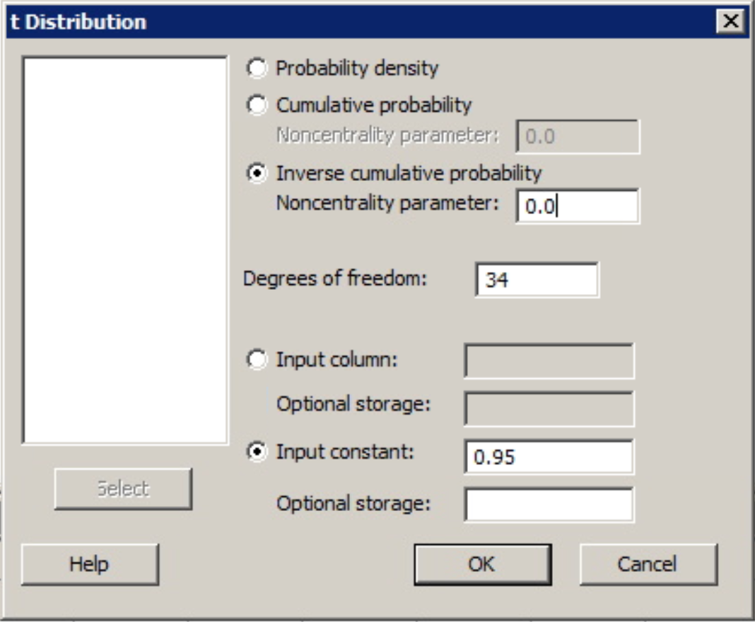
Minitab window for the t -distribution

The output from Minitab gives us $t_{0.05}$ with df= 34 as 1.69092.

P (X $\le$ x)	x
0.95	1.69092

Find $t_{0.05}$ where the degree of freedom is 30.

The t-value for an $\alpha$ of .05 and df of 30 is 1.697.

df	0.40	0.25	0.10	0.05	0.025	0.01	0.005	0.001	.0005
...	...	...	...	...	...	...	...	...	...
27	0.256	0.684	1.314	1.703	2.052	2.473	2.771	3.421	3.690
28	0.256	0.683	1.313	1.701	2.048	2.467	2.763	3.408	3.674
29	0.256	0.683	1.311	1.699	2.045	2.462	2.756	3.396	3.659
30	0.256	0.683	1.310	1.697	2.042	2.457	2.750	3.385	3.646

Note! When the sample size is larger than 30, the t-values are not that different from the z-values. Thus, a crude estimate for $t_{0.05}$ with 34 degrees of freedom is $z_{0.05} = 1.645$. Although it is a crude estimate, when software is available, it is best to find the $t$ values rather than use the $z$.

5.4.3 - Example

Example 5-6: Emergency Room Wait Time

You are interested in the average emergency room (ER) wait time at your local hospital. You take a random sample of 50 patients who visit the ER over the past week. From this sample, the mean wait time was 30 minutes and the standard deviation was 20 minutes. Find a 95% confidence interval for the average ER wait time for the hospital.

Answer

Is the population data normal? We don't know. However, the sample size is 50 which exceeds our minimum requirement of 30 in order to use the t-interval.

The population standard deviation is unknown; we only know the sample standard deviation. Having satisfied the conditions we proceed by finding the proper multiplier from the t-table. With n of 50 the d.f. are 49, and for 95% confidence, the alpha value is 5% or 0.05. From the t-table under the column 0.025 (remember we use α/2) and a d.f. of 40 (since 49 is not on the table), we arrive at a t-value of 2.021 Completing our confidence interval formula,\begin{align} &=\bar{x}\pm t_{\alpha/2}\dfrac{s}{\sqrt{n}}\\ &=30\pm 2.021\dfrac{20}{\sqrt{50}}\\ &=30\pm 5.72\\ &=(24.28, 35.72) \end{align}

Note that, $t_{0.025,49}\approx z_{0.025}$ as the degrees of freedom is 49

We are 95% confident that mean emergency room wait time at our local hospital is from 24.28 minutes to 35.72 minutes.

Find the CI for a population mean in Minitab:

In Minitab choose Stat > Basic Statistics > 1-Sample t .
From the drop down box select the Summarized data option button. (If you have the raw data you would use the default drop down of One or more samples, each in a column.)
Enter the sample size, sample mean, and sample standard deviation in their respective text boxes.
Click the Options button. The default confidence level is 95. If your desire another confidence level edit appropriately.
Click OK and OK again.

Using Minitab: Emergency Room Wait Time Example

Referring to our prior example of average emergency room wait time from our discussion on confidence intervals for a population mean, our by-hand calculations produced a 95% confidence interval of 24.28 to 35.72 minutes. Recall the following for that example: sample size 50, sample mean 30, and sample standard deviation 20.

Answer

SampleText

In Minitab following the above steps, we get a 95% confidence interval:

N	Mean	StDev	SE Mean	95% CI
50	30.00	20.00	2.84	(24.32, 35.68)

The slight discrepancy between the estimates is due to our by-hand calculation using the t-value associated with 40 degrees of freedom since the table did not include a d.f. of 49. Minitab used a t-value for the actually 49 degrees of freedom. With the larger degrees of freedom comes a smaller t-value. This would result in a smaller margin of error and a narrower interval - precisely what we have here.

The mean length of certain construction lumber is supposed to be 8.5 feet. A random sample of 81 pieces of such lumber gives a sample mean of 8.3 feet and a sample standard deviation of 1.2 feet.

What is the 95% CI for "mean length of such lumber?"

Step 1: Check the conditions: The sample size is large ($n\ge 30$), so we may continue using the value from the t-distribution as our multiplier.
Step 2: Construct the CI: The degrees of freedom are $n-1=80$. If we use the table, with d.f of 60, $t_{0.025}=2$.
The 95% confidence interval is \begin{align} &=\bar{x}\pm t_{0.025}\dfrac{s}{\sqrt{n}}\\ &=8.3\pm 2\dfrac{1.2}{\sqrt{81}}\\ &=8.3\pm 0.2667\\ &=(8.0333, 8.5667) \end{align}

What is the 99% CI for "mean length of such lumber?"

Step 1: Check the conditions: The sample size is large ($n\ge 30$), so we may continue using the value from the t-distribution as our multiplier.
Step 2: Construct the CI: The degrees of freedom are $n-1=80$. If we use the table, with d.f of 60, $t_{0.005}=2.66$. The 99% confidence interval is \begin{align} &=\bar{x}\pm t_{0.005}\dfrac{s}{\sqrt{n}}\\ &=8.3\pm 2.66\dfrac{1.2}{\sqrt{81}}\\ &=8.3\pm 0.3547\\ &=(7.9453, 8.6547) \end{align}

Reflecting back on interpretation of a proportion interval, we see the same basic structure: level of confidence, parameter of interest, lower and upper bounds.

5.4.4 - Checking Normality

Using Normal Probability Plot to Check Normality

If the sample size is less than 30, one needs to use a Normal Probability Plot to check whether the assumption that the data come from a normal distribution is valid.

Normal Probability Plot: The Normal Probability Plot is a graph that allows us to assess whether or not the data comes from a normal distribution.

Note! This plot should be used as a guide for us to assess if the assumption that the data come from a normal distribution is valid or not. It should not be used to “test” an assumption.

Example 5-7: Rattlesnake Lengths

It is very time consuming to find rattlesnakes and nerve racking to measure them (for obvious reasons). A scientist randomly finds 12 snakes from the central Pennsylvania area and measures their length. The following twelve measurements in inches are obtained:

40.2, 43.1, 45.5, 44.5, 39.5, 38.5, 40.2, 41.0, 41.6, 43.1, 44.9, 42.8

Using the above data, find a 90% confidence interval for the mean length of rattlesnakes in the central Pennsylvania area.

Answer

Step 1 Check Conditions

Think about what conditions you need to check. The sample size is only 12. The scenario does not give us an indication that the lengths follow a normal distribution. Therefore, let's do a normal probability plot to check whether the assumption that the data come from a normal distribution is valid.

Minitab: Creating a normal probability plot

To create a normal probability plot in Minitab:

Enter the 12 measurements into one column (name it length for this example) or upload the snakes.txt file.
Type or upload the data in the first column in Minitab.
Choose Graph > Probability Plot

Here is the normal probability plot for the rattlesnake data. What do you conclude about whether they may come from a normal distribution?

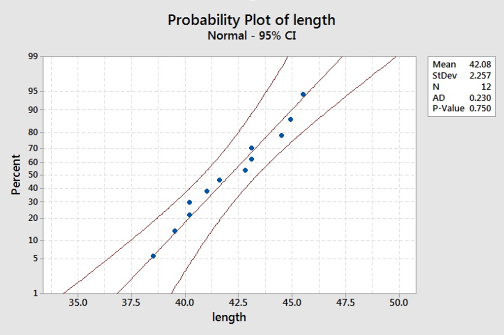
Minitab output of the normality plot for the snake example.

Since the points all fall within the confidence limits, it is reasonable to suggest that the data come from a normal distribution.

Step 2 Construct the CI

Now, we can proceed to find the 90% t-interval for the mean length of rattlesnakes in the central Pennsylvania area since even though the sample size is less than 30, the normality plot shows that the data may come from a normal distribution.

Minitab: Find the t-interval using Minitab

Enter the 12 measurements into one column (name it length for this example)
Choose Stat > Basic Statistics > 1-Sample t
Click on the variable (length for this example) and change to the desired confidence level

The Minitab output will provide the confidence interval. We get the following:

`N`	`Mean`	`StDev`	`SE Mean`	`90% CI`
`12`	`42.075`	`2.257`	`0.652`	`(40.905, 43.245)`

View the video to see these steps within Minitab.

Video: Minitab: 90% Confidence Interval for Continuous Data in Minitab

Step 3 Interpret the Interval

We are 90% confident that the population mean lengths of rattlesnakes is between 40.905 and 43.245 inches.

5.4.5 - Sample Size Computation

Sample Size Computation for the Population Mean Confidence Interval

Recall that a $(1-\alpha)$100% confidence interval for $\mu$ is $\bar{x}\pm t_{\alpha/2}\dfrac{s}{\sqrt{n}}$ where the multiplier $t$ has a t-distribution with $df = n - 1$. Thus, the margin of error, E, is equal to:

$E=t_{\alpha/2}\dfrac{s}{\sqrt{n}}$

To determine the sample size, one first decides the confidence level and the half width of the interval one wants. Then we can find the sample size to yield an interval with that confidence level and with a half width not more than the specified one. The crude method to find the sample size: $n=\left(\dfrac{z_{\alpha/2}\sigma}{E}\right)^2$ Then round up to the next whole integer.

Example 5-8: Spring Break

A marketing research firm wants to estimate the average amount a student spends during the Spring break. They want to determine it to within \$120 with 90% confidence. One can roughly say that it ranges from \$100 to \$1700. How many students should they sample?

Answer

To use the formula, we need all the pieces for $n=\left(\dfrac{z_{\alpha/2}\sigma}{E}\right)^2$. We know that $z_{\alpha/2}=1.645$ (for 90%). The margin of error, $E$, is 120. The only piece missing is $\sigma$. Since the standard deviation is not given in the problem, we can estimate it using $\dfrac{\text{range}}{4}$ from Lesson 1. Therefore, $\sigma=\dfrac{1700-100}{4}=400$. So we have...

\begin{align} n &=\left(\dfrac{1.645(400)}{120}\right)^2\\ &=30.07 \end{align}

Therefore, a sample of size $n=31$ is required.

Note! In homework and exams, it is fine if you simply use the cruder method. A more accurate method is provided in the following for your reference only.

The Iterative Method

A more accurate method to estimate the sample size: iteratively evaluate the formula since the t value also depends on n.

$n=\left(\dfrac{t_{\alpha/2}s}{E}\right)^2$

Use the example above for illustration. Start with an initial guess for $n$, plug in the formula, and iteratively solve for $n$.

If the initial guess for $n$ is 20, $t_{0.05} = 1.729$ and degrees of freedom = 19,

$n=\left(\dfrac{t_{\alpha/2}s}{E}\right)^2=n=\left(\dfrac{1.729(400)}{120}\right)^2=33.21$

For $n = 34$, degree of freedom = 33, and $t_{0.05} = 1.697$

$n=\left(\dfrac{t_{\alpha/2}s}{E}\right)^2=n=\left(\dfrac{1.697(400)}{120}\right)^2=31.99$

If we use $n = 32$, the result is the same. Thus, the more accurate answer to the example is to sample 32 students.

^[1]	Link
↥	Has Tooltip/Popover
	Toggleable Visibility

5.4 - Inference for the Population Mean

Overview

Point Estimates for a Population Mean

5.4.1 - Construct and Interpret the CI

Constructing a Confidence Interval for the Population Mean

Case 1: $\sigma$ is known

Note!

Case 2: \(\sigma\) is unknown

Constructing the Confidence Interval

What if the conditions are not met?

5.4.2 - The t-distribution

Properties of the t-distribution

Example 5-5: Finding t-values

5.4.3 - Example

Example 5-6: Emergency Room Wait Time

Answer

Using Minitab: Emergency Room Wait Time Example

5.4.4 - Checking Normality

Using Normal Probability Plot to Check Normality

Example 5-7: Rattlesnake Lengths

Step 1 Check Conditions

Minitab: Creating a normal probability plot

Step 2 Construct the CI

Minitab: Find the t-interval using Minitab

Video: Minitab: 90% Confidence Interval for Continuous Data in Minitab

Step 3 Interpret the Interval

5.4.5 - Sample Size Computation

Sample Size Computation for the Population Mean Confidence Interval

Example 5-8: Spring Break

Answer

The Iterative Method