Lesson 6b: Hypothesis Testing for One-Sample Mean
Lesson 6b: Hypothesis Testing for One-Sample MeanOverview
In the previous Lesson, we learned how to perform a hypothesis test for one proportion. The concepts of hypothesis testing remain constant for any hypothesis test. In these next few sections, we will present the hypothesis test for one mean. We start with our knowledge of the sampling distribution of the sample mean.
Recall that under certain conditions, the sampling distribution of the sample mean, \(\bar{x} \), is approximately normal with mean, \(\mu \), standard error \(\frac{\sigma}{\sqrt{n}} \), and estimated standard error \(\frac{s}{\sqrt{n}} \).
The conditions are:
- The distribution of the population is Normal
- The sample size is large \( n>30 \).
If at least one of conditions are satisfied, then...
\( t=\dfrac{\bar{x}-\mu_0}{\frac{s}{\sqrt{n}}} \)
will follow a t-distribution with \(n-1 \) degrees of freedom.
We can use this information to make probability statements for \(\bar{x} \).
Let’s look at an example.
Application
Length of Lumber
The mean length of the lumber is supposed to be 8.5 feet. A builder wants to check whether the shipment of lumber she receives has a mean length different from 8.5 feet. If the builder observes that the sample mean of 61 pieces of lumber is 8.3 feet with a sample standard deviation of 1.2 feet. What will she conclude? Is 8.3 very different from 8.5?
This depends on the standard deviation of \(\bar{x} \) .
\begin{align} t^*&=\dfrac{\bar{x}-\mu}{\frac{s}{\sqrt{n}}}\\&=\dfrac{8.3-8.5}{\frac{1.2}{\sqrt{61}}}\\&=-1.3 \end{align}
Thus, we are asking if \(-1.3\) is very far away from zero, since that corresponds to the case when \(\bar{x}\) is equal to \(\mu_0 \). If it is far away, then it is unlikely that the null hypothesis is true and one rejects it. Otherwise, one cannot reject the null hypothesis.
How do we determine whether to reject the null hypothesis?
It depends on the level of significance \(\alpha \) (step 2 of conducting a hypothesis test), and the probability the sample data would produce the observed result. In the next section, we set up the six steps for a hypothesis test for one mean.
Objectives
- Perform hypothesis testing for a population mean using the p-value approach and the rejection region approach.
- Use confidence intervals to draw conclusions about two-sided tests.
6b.1 - Steps in Conducting a Hypothesis Test for \(\mu\)
6b.1 - Steps in Conducting a Hypothesis Test for \(\mu\)
Six Steps for Conducting a One-Sample Mean Hypothesis Test
Steps 1-3
Let's apply the general steps for hypothesis testing to the specific case of testing a one-sample mean.
- Step 1: Set up the hypotheses and check conditions.
-
One Mean t-test Hypotheses
Left-Tailed- \( H_0\colon \mu=\mu_0 \)
- \( H_a\colon \mu<\mu_0\)
Right-Tailed- \( H_0\colon \mu=\mu_0 \)
- \( H_a\colon \mu>\mu_0 \)
Two-Tailed- \( H_0: \mu=\mu_0 \)
- \( H_a: \mu\ne \mu_0 \)
Conditions: The data comes from an approximately normal distribution or the sample size is at least 30.
- Step 2: Decide on the significance level, \(\alpha \).
- Typically, 5%. If \(\alpha\) is not specified, use 5%.
- Step 3: Calculate the test statistic.
-
One Mean t-test: \( t^*=\dfrac{\bar{x}-\mu_0}{\frac{s}{\sqrt{n}}} \)
Rejection Region Approach
Steps 4-6
- Step 4: Find the appropriate critical values for the tests. Write down clearly the rejection region for the problem.
-
Normal curve with a left tailed test shaded. Reject \(H_0\) if \(t^* \le t_\alpha\)
Normal curve with a right tailed test shaded. Reject \(H_0\) if \(t^* \ge t_{1-\alpha}\)
Normal curve with a two-tailed test shaded Reject \(H_0\) if \(|t^*| \ge |t_{\alpha/2}|\)
- Step 5: Make a decision about the null hypothesis.
- Check to see if the value of the test statistic falls in the rejection region. If it does, then reject \(H_0 \) (and conclude \(H_a \)). If it does not fall in the rejection region, do not reject \(H_0 \).
- Step 6: State an overall conclusion.
P-Value Approach
Steps 4-6
- Step 4: Compute the appropriate p-value based on our alternative hypothesis.
-
- If \(H_a \) is right-tailed, then the p-value is the probability the sample data produces a value equal to or greater than the observed test statistic.
- If \(H_a \) is left-tailed, then the p-value is the probability the sample data produces a value equal to or less than the observed test statistic.
- If \(H_a \) is two-tailed, then the p-value is two times the probability the sample data produces a value equal to or greater than the absolute value of the observed test statistic.
Left-Tailed- \(P(t \le t^*)\)
Right-Tailed- \(P(t\ge t^*)\)
Two-Tailed- \(2\) x \(P(t \ge |t^*|)\)
- Step 5: Make a decision about the null hypothesis.
- If the p-value is less than the significance level, \(\alpha\), then reject \(H_0\) (and conclude \(H_a \)). If it is greater than the significance level, then do not reject \(H_0 \).
- Step 6: State an overall conclusion.
Example 6-7 Length of Lumber
Continuing with our lumber example, the mean length of the lumber is supposed to be 8.5 feet. A builder wants to check whether the shipment of lumber she receives has a mean length different from 8.5 feet. If the builder observes that the sample mean of 61 pieces of lumber is 8.3 feet with a sample standard deviation of 1.2 feet, what will she conclude? Conduct this test at a 1% level of significance.
Conduct the test using the Rejection Region approach and the p-value approach.
- Step 1: Set up the hypotheses and check conditions.
-
Set up the hypotheses (since the research hypothesis is to check whether the mean is different from 8.5, we set it up as a two-tailed test):
\( H_0\colon \mu=8.5 \) vs. \(H_a\colon \mu\ne 8.5 \)
Can we use the t-test? The answer is yes since the sample size of 61 is sufficiently large (greater than 30).
- Step 2: Decide on the significance level, \(\alpha \).
- According to the question, \(\alpha = 0.01 \).
- Step 3: Calculate the test statistic.
- \begin{align} t^*&=\dfrac{\bar{x}-\mu_0}{\frac{s}{\sqrt{n}}}\\&=\dfrac{8.3-8.5}{\frac{1.2}{\sqrt{61}}}\\&=-1.3 \end{align}
Steps 4-6
- Step 4: Find the appropriate critical values for the tests. Write down clearly the rejection region for the problem.
- From the table and with degrees of freedom of 61-1=60, the critical value is \(t_{\alpha/2}=t_{0.005}=2.660 \). The rejection region for the two-tailed test is given by:
\( t^*\le -2.660 \) or \(t^*\ge 2.660 \)
*Recall how to use to Minitab or t-table to find the t percentiles (Lesson 5.4) - Step 5: Make a decision about the null hypothesis.
- The observed t-value, or test statistic, is -1.3. Since \(t^* \) does not fall within the rejection region, we fail to reject \(H_0 \).
- Step 6: State an overall conclusion.
- With a test statistic of -1.3 and critical value of ± 2.660 at a 1% level of significance, we do not have enough statistical evidence to reject the null hypothesis. We conclude that there is not enough statistical evidence that indicates that the mean length of lumber differs from 8.5 feet.
- Step 4: Compute the appropriate p-value based on our alternative hypothesis.
- \begin{align} \text{p-value}&=2P(T>|t^*|)\\&=2P\left(T>\left|\frac{\bar{x}-\mu_0}{\frac{s}{\sqrt{n}}}\right|\right)\\&=2P\left(T>\left|\frac{8.3-8.5}{\frac{1.2}{\sqrt{61}}}\right|\right)\\&=2P(T>|-1.3|)\\&=2P(T>1.3) \end{align}.
- From the t-table going across the row for 60 degrees of freedom, we do not find a value equal to 1.3. Without software to find a more exact probability, the best we can do from the t-table is find a range. We do see that the value falls between 1.296 and 1.671. These two t-values correspond to right-tail probabilities of 0.1 and 0.05, respectively. Since 1.3 is between these two t-values, then it stands to reason that the probability to the right of 1.3 would fall between 0.05 and 0.1. Therefore, the p-value would be = 2×(0.05 and 0.1) or from 0.1 to 0.2.
- Step 5: Make a decision about the null hypothesis.
- With this range of possible p-values exceeding our 1% level of significance for the test, we fail to reject the null hypothesis.
- Step 6: State an overall conclusion.
- With a test statistic of - 1.3 and p-value between 0.1 to 0.2, we fail to reject the null hypothesis at a 1% level of significance since the p-value would exceed our significance level. We conclude that there is not enough statistical evidence that indicates that the mean length of lumber differs from 8.5 feet.
Try it!
Emergency Room Wait Time

The administrator at your local hospital states that on weekends the average wait time for emergency room visits is 10 minutes. Based on discussions you have had with friends who have complained on how long they waited to be seen in the ER over a weekend, you dispute the administrator's claim. You decide to test your hypothesis. Over the course of a few weekends, you record the wait time for 40 randomly selected patients. The average wait time for these 40 patients is 11 minutes with a standard deviation of 3 minutes.
Do you have enough evidence to support your hypothesis that the average ER wait time exceeds 10 minutes? You opt to conduct the test at a 5% level of significance.
- Step 1: Set up the hypotheses and check conditions.
-
At this point we want to check whether we can apply the central limit theorem. The sample size is greater than 30, so we should be okay.
This is a right-tailed test.
\( H_0\colon \mu=10 \) vs \(H_a\colon \mu>10 \)
- Step 2: Decide on the significance level, \(\alpha \).
- The problem states that \(\alpha=0.05 \).
- Step 3: Calculate the test statistic.
- \begin{align} t^*&=\dfrac{\bar{x}-\mu_0}{\frac{s}{\sqrt{n}}}\\&=\dfrac{11-10}{\frac{3}{\sqrt{40}}}\\&=2.11 \end{align}
Steps 4-6
- Step 4: Find the appropriate critical values for the tests. Write down clearly the rejection region for the problem.
- The degrees of freedom for this test are \(n-1=40-1=39 \). The alternative is right-tailed. Therefore, we want to find the value, \(t_{0.05} \), such that \(P(T\ge t_{0.05})=0.05 \).
Using the table from the text, it shows 35 and 40 degrees of freedom. We would use 35 degrees of freedom. With \(\alpha=0.05 \) , we see a value of 1.69. The critical value is 1.69 and the rejection region is any \(t^* \) such that \(t^*\ge 1.69 \) .
Note! If we used software (discussed in the next section), we will find the critical value to be 1.685.
- Step 5: Make a decision about the null hypothesis.
- Our test statistic, 2.11, is greater than our critical value of 1.69 and therefore is in the rejection region. We would reject the null hypothesis.
- Step 6. State the conclusion in words.
- There is enough evidence, at a significance level of 5%, to reject the null hypothesis and conclude that the mean waiting time is greater than 10 minutes.
- Step 4: Compute the appropriate p-value based on our alternative hypothesis.
- Again, using the table with 35 degrees of freedom, our test statistic is 2.11 and is between 2.030 and 2.438. This corresponds to a p-value between 0.01 and 0.025.
Note! If we use software, the p-value is 0.0207.
- Step 5: Make a decision about the null hypothesis.
- Since our p-value is between 0.01 and 0.025, we know it is less than our significance level, 5%. Therefore, we reject the null hypothesis.
- Step 6: State an overall conclusion.
- There is enough evidence, at a significance level of 5%, to reject the null hypothesis and conclude that the mean waiting time is greater than 10 minutes.
6b.2 - Minitab: One-Sample Mean Hypothesis Test
6b.2 - Minitab: One-Sample Mean Hypothesis TestMinitab® – Conduct a One-Sample Mean t-Test
Note that these steps are very similar to those for one-mean confidence interval. The differences occur in steps 4 through 8.
To conduct the one sample mean t-test in Minitab...
- Choose Stat > Basic Stat > 1 Sample t.
- In the drop-down box use "One or more samples, each in a column" if you have the raw data, otherwise select "Summarized data" if you only have the sample statistics.
- If using the raw data, enter the column of interest into the blank variable window below the drop down selection. If using summarized data, enter the sample size, sample mean, and sample standard deviation in their respective fields.
- Choose the check box for "Perform hypothesis test" and enter the null hypothesis value.
- Choose Options.
- Enter the confidence level associated with alpha (e.g. 95% for alpha of 5%).
- From the drop down list for "Alternative hypothesis" select the correct alternative.
- Click OK and OK.
Minitab®
Example 6-8: Emergency Room Wait Time

Recall our emergency room wait time example where an administrator at your local hospital states that on weekends the average wait time for emergency room visits is 10 minutes. From our random sample of 40 patients, the average wait time for these 40 patients was 11 minutes with a standard deviation of 3 minutes. We conducted the test at a 5% level of significance and wanted to demonstrate that the average time exceeded 10 minutes. Also, recall in that example we found by hand a test statistic of t* = 2.11 and p-value with a range between 0.01 to 0.025
Our hypotheses were: \(H_0 \colon \mu=10\) and \(H_a\colon \mu>10\)
Conduct the same test using Minitab.
Answer
Using Minitab...
- Select Stat > Basic Stat > 1 Sample t.
- Choose the summarized data option and enter 40 for "Sample size", 11 for the "Sample mean", and 3 for the "Standard deviation".
- Check the box for "Perform Hypothesis Test" and enter the null value of 10
- Click Options .
- With our stated alpha value of 5% we keep the default confidence level of 95.
- Select "Mean> hypothesized mean" from the "Alternative Hypothesis" list.
- Click OK and OK again.
The output is:
One-Sample T
Test of \(\mu\) = 10 vs \(\mu\) > 10
| N | Mean | StDev | SE Mean | 95% Lower Bound | T | P |
|---|---|---|---|---|---|---|
| 40 | 11.000 | 3.000 | 0.474 | 10.201 | 2.11 | 0.021 |
Again, as the output indicates, our hand calculations were quite good. Notice that Minitab provides a more exact p-value of 0.021 which corresponds to our results as it falls within our calculated range of 0.01 to 0.025.
Minitab®
Finding Exact Critical Value for a One-Sample Mean t-Test
Since the t-table is not as detailed as the z-table, we can only estimate the critical value when the degrees of freedom are not found on the table. In order to obtain the exact critical value to use in order to conduct the rejection region approach, we can use a statistical package such as Minitab.
Minitab commands to obtain critical value:
- Calc > Probability Distributions > t-distribution
- Choose the radio button for 'Inverse Cumulative Distribution' (this finds the t-value that produces the entered probability to the left of it).
- Enter the correct degrees of freedom
- Choose the radio button for 'Input constant' and enter the alpha value (if one-side alternative) or alpha/2 (if two-sided alternative).
- Click Ok
Minitab®
6-8 Cont'd...

Find the exact critical value for our emergency room example. Recall by hand that we had to use the row with 35 degrees of freedom instead of the correct df of 39. In that example our critical value for alpha of 5% was 1.69.
- Go to Calc > Probability Distributions > t-distribution .
- Choose the radio button for 'Inverse Cumulative Distribution.'
- Enter 39 for 'degrees of freedom.'
- Choose the radio button for 'Input Constant' and enter 0.05
The output is as follows:
Student's t distribution with 39 DF
| P(X\(\le\)x) | x |
|---|---|
| 0.05 | -1.68488 |
This is where you need to be a little careful. Remember that our alternative was "greater than" or a right-tailed test. The output is the critical value for a left-tailed test. However, since the t-distribution is symmetrical, the area to the left of -1.68488 would be the same as the area to the right of 1.68488. Therefore, the critical value for out test with 39 degrees of freedom would be 1.68488, which doesn't differ much from the 1.69 we estimated using 35 degrees of freedom. This is why the table skips going one by one after 30; there is little difference between the values when increasing by only one degree of freedom.
6b.3 - Further Considerations for Hypothesis Testing
6b.3 - Further Considerations for Hypothesis TestingIn this section, we include a little more discussion about some of the issues with hypothesis tests and items to be concious about.
Committing an Error
Every time we make a decision and come to a conclusion, we must keep in mind that our decision is based on probability. Therefore, it is possible that we made a mistake.
Consider the example of the previous Lesson on whether the majority of Penn State students are from Pennsylvania. In that example, we took a random sample of 500 Penn State students and found that 278 are from Pennsylvania. We rejected the null hypothesis, at a significance level of 5% with a p-value of 0.006.
The significance level of 5% means that we have a 5% chance of committing a Type I error. That is, we have 5% chance that we rejected a true null hypothesis.
If we failed to reject a null hypothesis, then we could have committed a Type II error. This means that we could have failed to reject a false null hypothesis.
How Important are the Conditions of a Test?
In our six steps in hypothesis testing, one of them is to verify the conditions. If the conditions are not satisfied, we can still calculate the test statistic and find the rejection region (or p-value). We cannot, however, make a decision or state a conclusion. The conclusion is based on probability theory.
If the conditions are not satisfied, there are other methods to help us make a conclusion. The conclusion, however, may be based on other parameters, such as the median. There are other tests (some are discussed in later lessons) that can be used.
Statistical and Practical Significances
Our decision in the emergency room waiting times example was to reject the null hypothesis and conclude that the average wait time exceeds 10 minutes. However, our sample mean of 11 minutes wasn't too far off from 10. So what do you think of our conclusion? Yes, statistically there was a difference at the 5% level of significance, but are we "impressed" with the results? That is, do you think 11 minutes is really that much different from 10 minutes?
Since we are sampling data we have to expect some error in our results therefore even if the true wait time was 10 minutes it would be extremely unlikely for our sample data to have a mean of exactly 10 minutes. This is the difference between statistical significance and practical significance. The former is the result produced by the sample data while the latter is the practical application of those results.
Statistical significance is concerned with whether an observed effect is due to chance and practical significance means that the observed effect is large enough to be useful in the real world.
Critics of hypothesis-testing procedures have observed that a population mean is rarely exactly equal to the value in the null hypothesis and hence, by obtaining a large enough sample, virtually any null hypothesis can be rejected. Thus, it is important to distinguish between statistical significance and practical significance.
The Relationship Between Power, \(\beta\), and \(\alpha\)
Recall that \(\alpha \) is the probability of committing a Type I error. It is the value that is preset by the researcher. Therefore, the researcher has control over the probability of this type of error. But what about \(\beta \), the probability of a Type II error? How much control do we have over the probability of committing this error? Similarly, we want power, the probability we correctly reject a false null hypothesis, to be high (close to 1). Is there anything we can do to have a high power?
The relationship between power and \(\beta \) is an inverse relationship, namely...
Power \( =1-\beta \)
If we increase power, then we decrease \(\beta \). But how do increase power? One way to increase the power is to increase the sample size.
If the sample size is fixed, then decreasing \(\alpha \) will increase \(\beta \), and therefore decrease power. If one wants both \(\alpha \) and \(\beta \) to decrease, then one has to increase the sample size.
It is possible, using software, to find the sample size required for set values of \(\alpha \) and power. Also using software, it is possible to determine the value of power. We do not go into details on how to do this but you are welcome to explore on your own.
Gathering data is like tasting fine wine—you need the right amount. With wine, too small a sip keeps you from accurately assessing a subtle bouquet, but too large a sip overwhelms the palate.
We can’t tell you how big a sip to take at a wine-tasting event, but when it comes to collecting data, software tools can tell you how much data you need to be sure about your results.
6b.4 - More Examples
6b.4 - More ExamplesAs previously mentioned, setting up the hypotheses is the most important step. In this section, we provide some additional practice with examples where we do not indicate explicitly if it is a test for a mean or a proportion.
Try it!
Checkout Time
Fresh N Friendly food store advertises that their checkout waiting times is four minutes or less. An angry customer wants to dispute this claim. He takes a random sample of shoppers at the peak time and records their checkout times. Can he dispute their claim at significance level 10%?
Checkout times:
3.8, 5.3, 3.5, 4.5, 7.2, 5.1
- Step 1: Set up the hypotheses and check conditions.
-
The response variable is waiting time and is quantitative. Therefore, the hypotheses should be in terms of the population mean.
\( H_0\colon \mu=4 \) vs \(H_a\colon \mu>4 \)
The sample size is small, \(n=6 \). There is also no indication in the problem that the waiting times follow a normal distribution. We can use the Normal Probability Plot to examine the data.
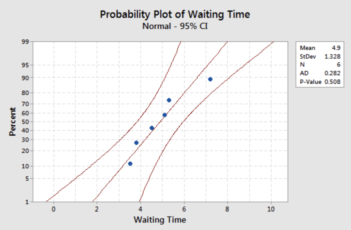
The data seem consistent with the Normal distribution and therefore it seems reasonable that the data come from a Normal distribution. We should use caution here, however. If the data do not come from a Normal distribution, the conclusion is not valid.
- Step 2: Decide on the significance level, \(\alpha \).
- The problem suggests that we use \(\alpha=0.10 \) .
- Step 3: Calculate the test statistic:
- In order to do so, we must first calculate the sample mean and sample standard deviation. The sample mean is \(\bar{x}=4.9 \) and \(s=1.3282 \). The test statistic is:
\begin{align} \text{t}^*&=\dfrac{\bar{x}-\mu_0}{\frac{s}{\sqrt{n}}}\\&=\dfrac{4.9-4}{\frac{1.3282}{\sqrt{6}}}\\&=1.6598 \end{align}
- Step 4: Compute the appropriate p-value based on our alternative hypothesis.(p-value approach)
- For this example, we will find the p-value. For extra practice, find the rejection region on your own. \begin{align} \text{p-value}&=P(T>t^*)\\&=P(T>1.6598)\\&=1-0.9211\\&=0.0789 \end{align} Where T is a t-distribution with \(n-1=6-1=5 \) degrees of freedom.
- Step 5: Make a decision about the null hypothesis.
- Since our p-value of 0.0789 is less than our significance level of 10%, we reject the null hypothesis.
- Step 6: State an overall conclusion.
- At 10% significance, we have enough evidence in the data to dispute the store’s claim that the mean waiting time is less than four minutes.
Try it!
Satisfaction Surveys
The CEO of a large computer company claims that 80 percent of his customers are “very satisfied” with the customer service they receive. To test this claim, the researcher surveyed 100 customers and 75 of them stated they are “very satisfied.” Based on these findings, can we reject the CEO's hypothesis that 80% of the customers are very satisfied?
- Step 1: Set up the hypotheses and check conditions.
-
The response is categorical so the hypotheses will be based on the population proportion. The claim, or the null, will be that the proportion is 0.8 and the alternative is that it is different than 0.8. In symbols we have:
\( H_0\colon p=0.8 \) vs \(H_a\colon p\ne 0.8 \)
The conditions, \(np_0=100(0.8) \) and \(n(1-p_0)=100(1-0.8) \) are both greater than five. Therefore, we can continue with the one proportion Z-test.
- Step 2: Decide on the significance level, \(\alpha \).
- The level of significance is not stated in the problem. If it is not stated, we typically assume it to be 5%.
- Step 3: Calculate the test statistic.
- The test statistic is:
\begin{align} \text{z}^*&=\dfrac{\hat{p}-p_0}{\sqrt{\frac{p_0(1-p_0)}{n}}}\\&=\dfrac{\frac{75}{100}-0.8}{\sqrt{\frac{0.8(1-0.8)}{100}}}\\&=-1.25 \end{align}
- Step 4: Compute the appropriate p-value based on our alternative hypothesis.(p-value approach).
- For this example we will use the p-value approach. You may want to find the critical value and rejection region for extra practice. \begin{align} \text{p-value}&=2P(Z>|z^*|)\\&=2P(Z>1.25)\\&=2(0.1056)\\&=0.2112 \end{align}
- Step 5: Make a decision about the null hypothesis.
- Since our p-value is greater than our significance level, we fail to reject the null hypothesis.
- Step 6: State an overall conclusion.
- At significance level of 5%, there is not enough evidence in the data to suggest the population proportion of customers who are “very satisfied” is not equal to 80%.
Try it!
Hotel Survey
There is a claim that about 10% of all men traveling on business bring a friend or a spouse. According to a survey by Rest Easy Hotel, 5% of the 40 men who are traveling for business purposes brought a friend or spouse. Can Rest Easy Hotel dispute this claim and conclude that it is not 10%?
- Step 1: Set up the hypotheses and check conditions.
-
The response variable is categorical (bring spouse or not). Our hypotheses will be based on the population proportion.
\(H_0\colon p=0.10 \text{ vs } H_a\colon p\ne0.1\)
Before we proceed, we need to check our conditions. We need \(np_0>5\) and \(n(1-p_0)>5\) and in this case we have \(40(0.10)=4\) and \(40(0.9)=36\).
- Since out conditions are not satisfied, we should not proceed with the Z-test for one proportion. It would be best to continue exact methods. We leave out how to do this.
6b.5 - Lesson 6b Summary
6b.5 - Lesson 6b SummaryThe concepts, logic, and terminology of hypothesis testing can take some time to master. It is worth it! Hypothesis testing is a very powerful statistical tool.
In this lesson, we covered how to set up the null and alternative hypotheses and how we can conclude to reject the null hypothesis or fail to reject the null. We also discussed the types of errors we can make and their respective probabilities.
We discussed how to apply our knowledge of sampling distributions to develop a test for a population parameter. We show how to complete the six steps for hypothesis testing for the population mean and the population proportion.
Next, we will move onto situations where we compare more than one population parameter.