Lesson 7: Comparing Two Population Parameters
Lesson 7: Comparing Two Population ParametersOverview
So far in our course, we have only discussed measurements taken in one variable for each sampling unit. This is referred to as univariate data. In this lesson, we are going to talk about measurements taken in two variables for each sampling unit. This is referred to as bivariate data.
Often when there are two measurements taken on the same sampling unit, one variable is the response variable and the other is the explanatory variable. The explanatory variable can be seen as the indicator of which population the sampling unit comes from. It helps to be able to identify which is the response and which is the explanatory variable.
In this lesson, here are some of the cases we will consider:
Two-Sample Cases
-
Categorical - taken from two distinct groups
- If the measurements are categorical and taken from two distinct groups, the analysis will involve comparing two independent proportions.
Sex and whether they smoke
Consider a case where we measure sex and whether they smoke. In this case, the response variable is categorical, and the explanatory variable is also categorical.
- Response variable: Yes or No to the Question “Do you smoke?”
- Explanatory variable: Sex (Female or Male)
-
Quantitative - taken from two distinct groups
- If the measurements are quantitative and taken from two distinct groups, the analysis will involve comparing two independent means.
GPA and the current degree level of a student
In this case, the response variable is quantitative, and the explanatory variable is categorical.
- Response variable: GPA
- Explanatory variable: Graduate or Undergraduate
-
Quantitative - taken twice from each subject (paired)
- If the measurements are quantitative and taken twice from each subject, the analysis will involve comparing two dependent means.
Dieting and the participant's weight before and after
In this case, the response is quantitative, and we will show later why there is no explanatory variable.
- Response variable: Weight
- Explanatory variable: Diet
-
Categorical - taken twice from each subject (paired)
- Finally, if the measurements are categorical and taken twice from each subject, the analysis will involve comparing two dependent proportions. However, we will not discuss this last situation.
To begin, just as we did previously, one has to first decide whether the problem you are investigating requires the analysis of categorical or quantitative data. In other words, you need to identify your response variable and determine the type of variable. Next, one has to determine if the two measurements are from independent samples or dependent samples.
You will find that much of what we discuss will be an extension of our previous lessons on confidence intervals and hypothesis testing for one-proportion and one-mean. We will want to check the necessary conditions in order to use the distributions as before. If conditions are satisfied, we calculate the specific test statistic and again compare this to a critical value (rejection region approach) or find the probability of observing this test statistic or one more extreme (p-value approach). The decision process will be the same as well: if the test statistic falls in the rejection region, we will reject the null hypothesis; if the p-value is less than the preset level of significance, we will reject the null hypothesis. The interpretation of confidence intervals in support of the hypothesis decision will also be familiar:
- if the interval does not contain the null hypothesis value, then we will reject the null hypothesis;
- if the interval contains the null hypothesis value, then we will fail to reject the null hypothesis.
One departure we will take from our previous lesson on hypothesis testing is how we will treat the null value. In the previous lesson, the null value could vary. In this lesson, when comparing two proportions or two means, we will use a null value of 0 (i.e., "no difference").
For example, \(\mu_1-\mu_2=0\) would mean that \(\mu_1=\mu_2\), and there would be no difference between the two population parameters. Similarly for two population proportions.
Although we focus on the difference equalling zero, it is possible to test for specific values of the difference using the methods presented. However, most applications research only for a difference in the parameters (i.e., the difference is less than, greater than, or not equal to zero).
We will start by comparing two independent population proportions, move to compare two independent population means, from there to paired population means, and ending with the comparison of two independent population variances.
Objectives
- Compare two population proportions using confidence intervals and hypothesis tests.
- Distinguish between independent data and paired data for when analyzing means.
- Compare two means from independent samples using confidence intervals and hypothesis tests when the variances are assumed equal.
- Compare two means from independent samples using confidence intervals and hypothesis tests when the variances are assumed unequal.
- Compare two means from dependent samples using confidence intervals and hypothesis tests.
- Compare two population variances using a hypothesis test.
7.1 - Difference of Two Independent Normal Variables
7.1 - Difference of Two Independent Normal VariablesIn the previous Lessons, we learned about the Central Limit Theorem and how we can apply it to find confidence intervals and use it to develop hypothesis tests. In this section, we will present a theorem to help us continue this idea in situations where we want to compare two population parameters.
As we mentioned before, when we compare two population means or two population proportions, we consider the difference between the two population parameters. In other words, we consider either \(\mu_1-\mu_2\) or \(p_1-p_2\).
We present the theory here to give you a general idea of how we can apply the Central Limit Theorem. We intentionally leave out the mathematical details.
Let \(X\) have a normal distribution with mean \(\mu_x\), variance \(\sigma^2_x\), and standard deviation \(\sigma_x\).
Let \(Y\) have a normal distribution with mean \(\mu_y\), variance \(\sigma^2_y\), and standard deviation \(\sigma_y\).
If \(X\) and \(Y\) are independent, then \(X-Y\) will follow a normal distribution with mean \(\mu_x-\mu_y\), variance \(\sigma^2_x+\sigma^2_y\), and standard deviation \(\sqrt{\sigma^2_x+\sigma^2_y}\).
The idea is that, if the two random variables are normal, then their difference will also be normal. This is wonderful but how can we apply the Central Limit Theorem?
If \(X\) and \(Y\) are normal, we know that \(\bar{X}\) and \(\bar{Y}\) will also be normal. If \(X\) and \(Y\) are not normal but the sample size is large, then \(\bar{X}\) and \(\bar{Y}\) will be approximately normal (applying the CLT). Using the theorem above, then \(\bar{X}-\bar{Y}\) will be approximately normal with mean \(\mu_1-\mu_2\).
This is great! This theory can be applied when comparing two population proportions, and two population means. The details are provided in the next two sections.
7.2 - Comparing Two Population Proportions
7.2 - Comparing Two Population ProportionsIntroduction
When we have a categorical variable of interest measured in two populations, it is quite often that we are interested in comparing the proportions of a certain category for the two populations.
Let’s consider the following example.
Example: Received $100 by Mistake

Males and females were asked about what they would do if they received a $100 bill by mail, addressed to their neighbor, but wrongly delivered to them. Would they return it to their neighbor? Of the 69 males sampled, 52 said "yes" and of the 131 females sampled, 120 said "yes."
Does the data indicate that the proportions that said "yes" are different for male and female? How do we begin to answer this question?
If the proportion of males who said “yes, they would return it” is denoted as \(p_1\) and the proportion of females who said “yes, they would return it” is denoted as \(p_2\), then the following equations indicate that \(p_1\) is equal to \(p_2\).
\(p_1-p_2=0\) or \(\dfrac{p_1}{p_2}=1\)
We would need to develop a confidence interval or perform a hypothesis test for one of these expressions.
Moving forward
There may be other ways of setting up these equations such that the proportions are equal. We choose the difference due to the theory discussed in the last section. Under certain conditions, the sampling distribution of \(\hat{p}_1\), for example, is approximately normal and centered around \(p_1\). Similarly, the sampling distribution of \(\hat{p}_2\) is approximately normal and centered around \(p_2\). Their difference, \(\hat{p}_1-\hat{p}_2\), will then be approximately normal and centered around \(p_1-p_2\), which we can use to determine if there is a difference.
In the next subsections, we explain how to use this idea to develop a confidence interval and hypothesis tests for \(p_1-p_2\).
7.2.1 - Confidence Intervals
7.2.1 - Confidence IntervalsIn this section, we begin by defining the point estimate and developing the confidence interval based on what we have learned so far.
- Point Estimate
-
The point estimate for the difference between the two population proportions, \(p_1-p_2\), is the difference between the two sample proportions written as \(\hat{p}_1-\hat{p}_2\).
We know that a point estimate is probably not a good estimator of the actual population. By adding some amount of error to this point estimate, we can create a confidence interval as we did with one sample parameters.
Derivation of the Confidence Interval
Consider two populations and label them as population 1 and population 2. Take a random sample of size \(n_1\) from population 1 and take a random sample of size \(n_2\) from population 2. If we consider them separately,
- Proportion from Sample 1:
-
If \(n_1p_1\ge 5\) and \(n_1(1-p_1)\ge 5\), then \(\hat{p}_1\) will follow a normal distribution with...
\begin{array}{rcc} \text{Mean:}&&p_1 \\ \text{ Standard Error:}&& \sqrt{\dfrac{p_1(1-p_1)}{n_1}} \\ \text{Estimated Standard Error:}&& \sqrt{\dfrac{\hat{p}_1(1-\hat{p}_1)}{n_1}} \end{array}
- Proportion from Sample 2:
- If \(n_2p_2\ge 5\) and \(n_2(1-p_2)\ge 5\), then \(\hat{p}_2\) will follow a normal distribution with...
\begin{array}{rcc} \text{Mean:}&&p_2 \\ \text{ Standard Error:}&& \sqrt{\dfrac{p_2(1-p_2)}{n_2}} \\ \text{Estimated Standard Error:}&& \sqrt{\dfrac{\hat{p}_2(1-\hat{p}_2)}{n_2}} \end{array}
- Sample Proportion 1 - Sample Proportion 2:
-
Using the theory introduced previously, if \(n_1p_1\), \(n_1(1-p_1)\), \(n_2p_2\), and \(n_2(1-p_2)\) are all greater than five and we have independent samples, then the sampling distribution of \(\hat{p}_1-\hat{p}_2\) is approximately normal with...
\begin{array}{rcc} \text{Mean:}&&p_1-p_2 \\ \text{ Standard Error:}&& \sqrt{\dfrac{p_1(1-p_1)}{n_1}+\dfrac{p_2(1-p_2)}{n_2}} \\ \text{Estimated Standard Error:}&& \sqrt{\dfrac{\hat{p}_1(1-\hat{p}_1)}{n_1}+\dfrac{\hat{p}_2(1-\hat{p}_2)}{n_2}} \end{array}
Putting these pieces together, we can construct the confidence interval for \(p_1-p_2\). Since we do not know \(p_1\) and \(p_2\), we need to check the conditions using \(n_1\hat{p}_1\), \(n_1(1-\hat{p}_1)\), \(n_2\hat{p}_2\), and \(n_2(1-\hat{p}_2)\). If these conditions are satisfied, then the confidence interval can be constructed for two independent proportions.
- Confidence interval for two independent proportions
-
The \((1-\alpha)100\%\) confidence interval of \(p_1-p_2\) is given by:
\(\hat{p}_1-\hat{p}_2\pm z_{\alpha/2}\sqrt{\dfrac{\hat{p}_1(1-\hat{p}_1)}{n_1}+\dfrac{\hat{p}_2(1-\hat{p}_2)}{n_2}}\)
Example 7-1: Received $100 by Mistake

Males and females were asked about what they would do if they received a $100 bill by mail, addressed to their neighbor, but wrongly delivered to them. Would they return it to their neighbor? Of the 69 males sampled, 52 said "yes" and of the 131 females sampled, 120 said "yes."
Find a 95% confidence interval for the difference in proportions for males and females who said "yes."
Let’s let sample one be males and sample two be females. Then we have:
- Males:
- \(n_1=69\), \(\hat{p}_1=\dfrac{52}{69}\)
- Females:
- \(n_2=131\), \(\hat{p}_2=\dfrac{120}{131}\)
Checking conditions we see that \(n_1\hat{p}_1\), \(n_1(1-\hat{p}_1)\), \(n_2\hat{p}_2\), and \(n_2(1-\hat{p}_2)\) are all greater than five so our conditions are satisfied.
Using the formula above, we get:
\begin{array}{rcl} \hat{p}_1-\hat{p}_2 &\pm &z_{\alpha/2}\sqrt{\dfrac{\hat{p}_1(1-\hat{p}_1)}{n_1}+\dfrac{\hat{p}_2(1-\hat{p}_2)}{n_2}}\\ \dfrac{52}{69}-\dfrac{120}{131}&\pm &1.96\sqrt{\dfrac{\frac{52}{69}\left(1-\frac{52}{69}\right)}{69}+\dfrac{\frac{120}{131}(1-\frac{120}{131})}{131}}\\ -0.1624 &\pm &1.96 \left(0.05725\right)\\ -0.1624 &\pm &0.1122\ or \ (-0.2746, -0.0502)\\ \end{array}
We are 95% confident that the difference of population proportions of males who said "yes" and females who said "yes" is between -0.2746 and -0.0502.
Based on both ends of the interval being negative, it seems like the proportion of females who would return it is higher than the proportion of males who would return it.
We will discuss how to find the confidence interval using Minitab after we examine the hypothesis test for two proportion. Minitab calculates the test and the confidence interval at the same time.
Caution! What happens if we defined \(\hat{p}_1\) to be the proportion of females and \(\hat{p}_2\) for the proportion of males? If you follow through the calculations, you will find that the confidence interval will differ only in sign. In other words, if female was \(\hat{p}_1\), the interval would be 0.0502 to 0.2746. It still shows that the proportion of females is higher than the proportion of males.
7.2.2 - Hypothesis Testing
7.2.2 - Hypothesis TestingDerivation of the Test
We are now going to develop the hypothesis test for the difference of two proportions for independent samples. The hypothesis test will follow the same six steps we learned in the previous Lesson although they are not explicitly stated.
We will use the sampling distribution of \(\hat{p}_1-\hat{p}_2\) as we did for the confidence interval. One major difference in the hypothesis test is the null hypothesis and assuming the null hypothesis is true.
For a test for two proportions, we are interested in the difference. If the difference is zero, then they are not different (i.e., they are equal). Therefore, the null hypothesis will always be:
\(H_0\colon p_1-p_2=0\)
Another way to look at it is \(H_0\colon p_1=p_2\). This is worth stopping to think about. Remember, in hypothesis testing, we assume the null hypothesis is true. In this case, it means that \(p_1\) and \(p_2\) are equal. Under this assumption, then \(\hat{p}_1\) and \(\hat{p}_2\) are both estimating the same proportion. Think of this proportion as \(p^*\). Therefore, the sampling distribution of both proportions, \(\hat{p}_1\) and \(\hat{p}_2\), will, under certain conditions, be approximately normal centered around \(p^*\), with standard error \(\sqrt{\dfrac{p^*(1-p^*)}{n_i}}\), for \(i=1, 2\).
We take this into account by finding an estimate for this \(p^*\) using the two sample proportions. We can calculate an estimate of \(p^*\) using the following formula:
\(\hat{p}^*=\dfrac{x_1+x_2}{n_1+n_2}\)
This value is the total number in the desired categories \((x_1+x_2)\) from both samples over the total number of sampling units in the combined sample \((n_1+n_2)\).
Putting everything together, if we assume \(p_1=p_2\), then the sampling distribution of \(\hat{p}_1-\hat{p}_2\) will be approximately normal with mean 0 and standard error of \(\sqrt{p^*(1-p^*)\left(\frac{1}{n_1}+\frac{1}{n_2}\right)}\), under certain conditions.
Therefore,
\(z^*=\dfrac{(\hat{p}_1-\hat{p}_2)-0}{\sqrt{\hat{p}^*(1-\hat{p}^*)\left(\dfrac{1}{n_1}+\dfrac{1}{n_2}\right)}}\)
...will follow a standard normal distribution.
Finally, we can develop our hypothesis test for \(p_1-p_2\).
Null: \(H_0\colon p_1-p_2=0\)
Possible Alternatives:
\(H_a\colon p_1-p_2\ne0\)
\(H_a\colon p_1-p_2>0\)
\(H_a\colon p_1-p_2<0\)
Conditions:
\(n_1\hat{p}_1\), \(n_1(1-\hat{p}_1)\), \(n_2\hat{p}_2\), and \(n_2(1-\hat{p}_2)\) are all greater than five
The test statistic is:
\(z^*=\dfrac{\hat{p}_1-\hat{p}_2-0}{\sqrt{\hat{p}^*(1-\hat{p}^*)\left(\dfrac{1}{n_1}+\dfrac{1}{n_2}\right)}}\)
...where \(\hat{p}^*=\dfrac{x_1+x_2}{n_1+n_2}\).
The critical values, rejection regions, p-values, and decisions will all follow the same steps as those from a hypothesis test for a one sample proportion.
Example 7-2: Received $100 by Mistake

Let's continue with the question that was asked previously.
Males and females were asked about what they would do if they received a $100 bill by mail, addressed to their neighbor, but wrongly delivered to them. Would they return it to their neighbor? Of the 69 males sampled, 52 said “yes” and of the 131 females sampled, 120 said “yes.”
Does the data indicate that the proportions that said “yes” are different for males and females at a 5% level of significance? Conduct the test using the p-value approach.
Again, let’s define males as sample 1.
The conditions are all satisfied as we have shown previously.
The null and alternative hypotheses are:
\(H_0\colon p_1-p_2=0\) vs \(H_a\colon p_1-p_2\ne 0\)
The test statistic:
\(n_1=69\), \(\hat{p}_1=\frac{52}{69}\)
\(n_2=131\), \(\hat{p}_2=\frac{120}{131}\)
\(\hat{p}^*=\dfrac{x_1+x_2}{n_1+n_2}=\dfrac{52+120}{69+131}=\dfrac{172}{200}=0.86\)
\(z^*=\dfrac{\hat{p}_1-\hat{p}_2-0}{\sqrt{\hat{p}^*(1-\hat{p}^*)\left(\frac{1}{n_1}+\frac{1}{n_2}\right)}}=\dfrac{\dfrac{52}{69}-\dfrac{120}{131}}{\sqrt{0.86(1-0.86)\left(\frac{1}{69}+\frac{1}{131}\right)}}=-3.1466\)
The p-value of the test based on the two-sided alternative is:
\(\text{p-value}=2P(Z>|-3.1466|)=2P(Z>3.1466)=2(0.0008)=0.0016\)
Since our p-value of 0.0016 is less than our significance level of 5%, we reject the null hypothesis. There is enough evidence to suggest that proportions of males and females who would return the money are different.
Minitab: Inference for Two Proportions with Independent Samples
To conduct inference for two proportions with an independent sample in Minitab...
- Choose Stat > Basic Statistics > 2 proportions
The following window will appear. In the drop-down choose ‘Summarized data’ and entered the number of events and trials for both samples.
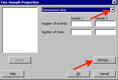
- Choose Options to display this window.
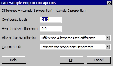
Notice how the difference is calculated. We also want to make sure that we are using the pooled estimate of the proportion as the test method. In Minitab, you need to get into options and select "Use pooled estimate of p for test." If you don't think that is reasonable to assume, then don't check the option.
You should get the following output for this example:
Test and CI for Two Proportions
| Sample | X | N | Sample p |
|---|---|---|---|
| 1 | 52 | 69 | 0.753623 |
| 2 | 120 | 131 | 0.916031 |
Difference = p (1) - p (2)
Estimate for difference: -0.162407
95% CI for difference: (-0.274625, -0.0501900)
Test for difference = 0 (vs ≠ 0): Z = -3.15 P-Value = 0.002 (Use this!)
Fisher's exact test: P-Value = 0.003 (Ignore the Fisher's exact test. This test uses a different method to calculate a test statistic from the Z-test we have learned in this lesson.)
Ignore the Fisher's p-value! The p-value highlighted above is calculated using the methods we learned in this lesson. The Fisher's test uses a different method than what we explained in this lesson to calculate a test statistic and p-value. This method incorporates a log of the ratio of observed to expected values. It's just a different technique that is more complicated to do by-hand. Minitab automatically includes both results in its output.
Try it!
In 1980, of 750 men 20-34 years old, 130 were found to be overweight. Whereas, in 1990, of 700 men, 20-34 years old, 160 were found to be overweight.
At the 5% significance level, do the data provide sufficient evidence to conclude that, for men 20-34 years old, a higher percentage were overweight in 1990 than 10 years earlier? Conduct the test using the p-value approach.
Let’s define 1990 as sample 1.
The null and alternative hypotheses are:
\(H_0\colon p_1-p_2=0\) vs \(H_a\colon p_1-p_2>0\)
\(n_1=700\), \(\hat{p}_1=\frac{160}{700}\)
\(n_2=750\), \(\hat{p}_2=\frac{130}{750}\)
\(\hat{p}^*=\dfrac{x_1+x_2}{n_1+n_2}=\dfrac{160+130}{700+750}=\dfrac{290}{1450}=0.2\)
The conditions are all satisfied: \(n_1\hat{p}_1\), \(n_1(1-\hat{p}_1)\), \(n_2\hat{p}_2\), and \(n_2(1-\hat{p}_2)\) are all greater than 5.
The test statistic:
\(z^*=\dfrac{\hat{p}_1-\hat{p}_2-0}{\sqrt{\hat{p}^*(1-\hat{p}^*)\left(\frac{1}{n_1}+\frac{1}{n_2}\right)}}=\dfrac{\dfrac{160}{700}-\dfrac{130}{750}}{\sqrt{0.2(1-0.2)\left(\frac{1}{700}+\frac{1}{750}\right)}}=2.6277\)
The p-value of the test based on the right-tailed alternative is:
\(\text{p-value}=P(Z>2.6277)=0.0043\)
Since our p-value of 0.0043 is less than our significance level of 5%, we reject the null hypothesis. There is enough evidence to suggest that the proportion of males overweight in 1990 is greater than the proportion in 1980.
Using Minitab
To conduct inference for two proportions with independent samples in Minitab...
- Choose Stat > Basic Statistics > 2 proportions
- Choose Options
-
Select "Difference > hypothesized difference" for 'Alternative Hypothesis.
You should get the following output.
Test and CI for Two Proportions
| Sample | X | N | Sample p |
|---|---|---|---|
| 1 | 160 | 700 | 0.228571 |
| 2 | 130 | 750 | 0.173333 |
Difference = p (1) - p (2)
Estimate for difference: 0.0552381
95% upper bound for difference: 0.0206200
Test for difference = 0 (vs < 0): Z = 2.62 P-Value = 0.004
Fisher's exact test: P-Value = 0.005 (Ignore the Fisher's exact test)
7.3 - Comparing Two Population Means
7.3 - Comparing Two Population MeansIntroduction
In this section, we are going to approach constructing the confidence interval and developing the hypothesis test similarly to how we approached those of the difference in two proportions.
There are a few extra steps we need to take, however. First, we need to consider whether the two populations are independent. When considering the sample mean, there were two parameters we had to consider, \(\mu\) the population mean, and \(\sigma\) the population standard deviation. Therefore, the second step is to determine if we are in a situation where the population standard deviations are the same or if they are different.
Independent and Dependent Samples
It is important to be able to distinguish between an independent sample or a dependent sample.
- Independent sample
- The samples from two populations are independent if the samples selected from one of the populations has no relationship with the samples selected from the other population.
- Dependent sample
- The samples are dependent (also called paired data) if each measurement in one sample is matched or paired with a particular measurement in the other sample. Another way to consider this is how many measurements are taken off of each subject. If only one measurement, then independent; if two measurements, then paired. Exceptions are in familial situations such as in a study of spouses or twins. In such cases, the data is almost always treated as paired data.
The following are examples to illustrate the two types of samples.
Example 7-3: Gas Mileage
We want to compare the gas mileage of two brands of gasoline. Describe how to design a study involving...
- independent sample
Answer: Randomly assign 12 cars to use Brand A and another 12 cars to use Brand B.
- dependent samples
Answer: Using 12 cars, have each car use Brand A and Brand B. Compare the differences in mileage for each car.
Try it!
- We want to compare whether people give a higher taste rating to Coke or Pepsi. To avoid a possible psychological effect, the subjects should taste the drinks blind (i.e., they don't know the identity of the drink). Describe how to design a study involving independent sample and dependent samples.
- Design involving independent samples
- Design involving dependent samples
- Answer: Randomly assign half of the subjects to taste Coke and the other half to taste Pepsi.
-
Answer: Allow all the subjects to rate both Coke and Pepsi. The drinks should be given in random order. The same subject's ratings of the Coke and the Pepsi form a paired data set.
- Compare the time that males and females spend watching TV.
- We randomly select 20 males and 20 females and compare the average time they spend watching TV. Is this an independent sample or paired sample?
- We randomly select 20 couples and compare the time the husbands and wives spend watching TV. Is this an independent sample or paired sample?
- Answer: Independent Sample
-
Answer: Paired sample
The two types of samples require a different theory to construct a confidence interval and develop a hypothesis test. We consider each case separately, beginning with independent samples.
7.3.1 - Inference for Independent Means
7.3.1 - Inference for Independent MeansTwo-Cases for Independent Means
As with comparing two population proportions, when we compare two population means from independent populations, the interest is in the difference of the two means. In other words, if \(\mu_1\) is the population mean from population 1 and \(\mu_2\) is the population mean from population 2, then the difference is \(\mu_1-\mu_2\). If \(\mu_1-\mu_2=0\) then there is no difference between the two population parameters.
If each population is normal, then the sampling distribution of \(\bar{x}_i\) is normal with mean \(\mu_i\), standard error \(\dfrac{\sigma_i}{\sqrt{n_i}}\), and the estimated standard error \(\dfrac{s_i}{\sqrt{n_i}}\), for \(i=1, 2\).
Using the Central Limit Theorem, if the population is not normal, then with a large sample, the sampling distribution is approximately normal.
The theorem presented in this Lesson says that if either of the above are true, then \(\bar{x}_1-\bar{x}_2\) is approximately normal with mean \(\mu_1-\mu_2\), and standard error \(\sqrt{\dfrac{\sigma^2_1}{n_1}+\dfrac{\sigma^2_2}{n_2}}\).
However, in most cases, \(\sigma_1\) and \(\sigma_2\) are unknown, and they have to be estimated. It seems natural to estimate \(\sigma_1\) by \(s_1\) and \(\sigma_2\) by \(s_2\). When the sample sizes are small, the estimates may not be that accurate and one may get a better estimate for the common standard deviation by pooling the data from both populations if the standard deviations for the two populations are not that different.
Given this, there are two options for estimating the variances for the independent samples:
- Using pooled variances
- Using unpooled (or unequal) variances
When to use which? When we are reasonably sure that the two populations have nearly equal variances, then we use the pooled variances test. Otherwise, we use the unpooled (or separate) variance test.
7.3.1.1 - Pooled Variances
7.3.1.1 - Pooled VariancesConfidence Intervals for \(\boldsymbol{\mu_1-\mu_2}\): Pooled Variances
When we have good reason to believe that the variance for population 1 is equal to that of population 2, we can estimate the common variance by pooling information from samples from population 1 and population 2.
An informal check for this is to compare the ratio of the two sample standard deviations. If the two are equal, the ratio would be 1, i.e. \(\frac{s_1}{s_2}=1\). However, since these are samples and therefore involve error, we cannot expect the ratio to be exactly 1. When the sample sizes are nearly equal (admittedly "nearly equal" is somewhat ambiguous, so often if sample sizes are small one requires they be equal), then a good Rule of Thumb to use is to see if the ratio falls from 0.5 to 2. That is, neither sample standard deviation is more than twice the other.
If this rule of thumb is satisfied, we can assume the variances are equal. Later in this lesson, we will examine a more formal test for equality of variances.
- Let \(n_1\) be the sample size from population 1 and let \(s_1\) be the sample standard deviation of population 1.
- Let \(n_2\) be the sample size from population 2 and \(s_2\) be the sample standard deviation of population 2.
Then the common standard deviation can be estimated by the pooled standard deviation:
\(s_p=\sqrt{\dfrac{(n_1-1)s_1^2+(n_2-1)s^2_2}{n_1+n_2-2}}\)
If we can assume the populations are independent, that each population is normal or has a large sample size, and that the population variances are the same, then it can be shown that...
\(t=\dfrac{\bar{x}_1-\bar{x_2}-0}{s_p\sqrt{\frac{1}{n_1}+\frac{1}{n_2}}}\)
follows a t-distribution with \(n_1+n_2-2\) degrees of freedom.
Now, we can construct a confidence interval for the difference of two means, \(\mu_1-\mu_2\).
- \(\boldsymbol{(1-\alpha)100\%}\) Confidence interval for \(\boldsymbol{\mu_1-\mu_2}\) for Pooled Variances
- \(\bar{x}_1-\bar{x}_2\pm t_{\alpha/2}s_p\sqrt{\frac{1}{n_1}+\frac{1}{n_2}}\)
-
where \(t_{\alpha/2}\) comes from a t-distribution with \(n_1+n_2-2\) degrees of freedom.
Hypothesis Tests for \(\boldsymbol{\mu_1-\mu_2}\): The Pooled t-test
Now let's consider the hypothesis test for the mean differences with pooled variances.
\(H_0\colon\mu_1-\mu_2=0\)
\(H_a\colon \mu_1-\mu_2\ne0\)
\(H_a\colon \mu_1-\mu_2>0\)
\(H_a\colon \mu_1-\mu_2<0\)
The assumptions/conditions are:
- The populations are independent
- The population variances are equal
- Each population is either normal or the sample size is large.
The test statistic is...
\(t^*=\dfrac{\bar{x}_1-\bar{x}_2-0}{s_p\sqrt{\frac{1}{n_1}+\frac{1}{n_2}}}\)
And \(t^*\) follows a t-distribution with degrees of freedom equal to \(df=n_1+n_2-2\).
The p-value, critical value, rejection region, and conclusion are found similarly to what we have done before.
Example 7-4: Comparing Packing Machines
In a packing plant, a machine packs cartons with jars. It is supposed that a new machine will pack faster on the average than the machine currently used. To test that hypothesis, the times it takes each machine to pack ten cartons are recorded. The results, (machine.txt), in seconds, are shown in the tables.
| 42.1 | 41.3 | 42.4 | 43.2 | 41.8 |
| 41.0 | 41.8 | 42.8 | 42.3 | 42.7 |
\(\bar{x}_1=42.14, \text{s}_1= 0.683\)
| 42.7 | 43.8 | 42.5 | 43.1 | 44.0 |
| 43.6 | 43.3 | 43.5 | 41.7 | 44.1 |
\(\bar{x}_2=43.23, \text{s}_2= 0.750\)
Do the data provide sufficient evidence to conclude that, on the average, the new machine packs faster?
Are these independent samples? Yes, since the samples from the two machines are not related.
Are these large samples or a normal population?
We have \(n_1\lt 30\) and \(n_2\lt 30\). We do not have large enough samples, and thus we need to check the normality assumption from both populations. Let's take a look at the normality plots for this data:
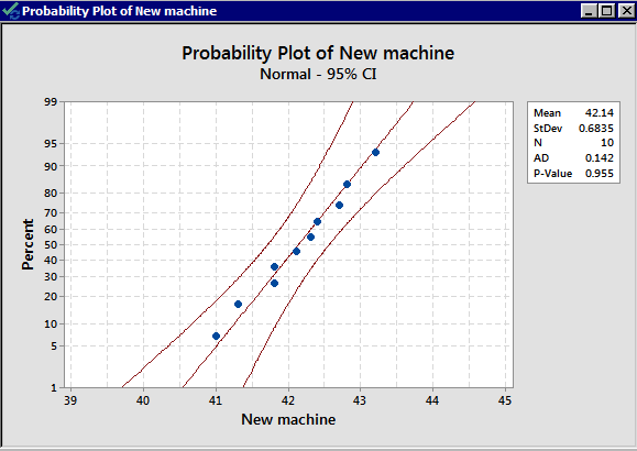
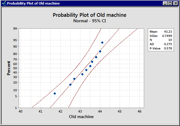
From the normal probability plots, we conclude that both populations may come from normal distributions. Remember the plots do not indicate that they DO come from a normal distribution. It only shows if there are clear violations. We should proceed with caution.
Do the populations have equal variance? No information allows us to assume they are equal. We can use our rule of thumb to see if they are “close.” They are not that different as \(\dfrac{s_1}{s_2}=\dfrac{0.683}{0.750}=0.91\) is quite close to 1. This assumption does not seem to be violated.
We can thus proceed with the pooled t-test.
Let \(\mu_1\) denote the mean for the new machine and \(\mu_2\) denote the mean for the old machine.
The null hypothesis is that there is no difference in the two population means, i.e.
\(H_0\colon \mu_1-\mu_2=0\)
The alternative is that the new machine is faster, i.e.
\(H_a\colon \mu_1-\mu_2<0\)
The significance level is 5%. Since we may assume the population variances are equal, we first have to calculate the pooled standard deviation:
\begin{align} s_p&=\sqrt{\frac{(n_1-1)s^2_1+(n_2-1)s^2_2}{n_1+n_2-2}}\\ &=\sqrt{\frac{(10-1)(0.683)^2+(10-1)(0.750)^2}{10+10-2}}\\ &=\sqrt{\dfrac{9.261}{18}}\\ &=0.7173 \end{align}
The test statistic is:
\begin{align} t^*&=\dfrac{\bar{x}_1-\bar{x}_2-0}{s_p\sqrt{\frac{1}{n_1}+\frac{1}{n_2}}}\\ &=\dfrac{42.14-43.23}{0.7173\sqrt{\frac{1}{10}+\frac{1}{10}}}\\&=-3.398 \end{align}
The alternative is left-tailed so the critical value is the value \(a\) such that \(P(T<a)=0.05\), with \(10+10-2=18\) degrees of freedom. The critical value is -1.7341. The rejection region is \(t^*<-1.7341\).
Our test statistic, -3.3978, is in our rejection region, therefore, we reject the null hypothesis. With a significance level of 5%, we reject the null hypothesis and conclude there is enough evidence to suggest that the new machine is faster than the old machine.
To find the interval, we need all of the pieces. We calculated all but one when we conducted the hypothesis test. We only need the multiplier. For a 99% confidence interval, the multiplier is \(t_{0.01/2}\) with degrees of freedom equal to 18. This value is 2.878.
The interval is:
\(\bar{x}_1-\bar{x}_2\pm t_{\alpha/2}s_p\sqrt{\frac{1}{n_1}+\frac{1}{n_2}}\)
\((42.14-43.23)\pm 2.878(0.7173)\sqrt{\frac{1}{10}+\frac{1}{10}}\)
\(-1.09\pm 0.9232\)
The 99% confidence interval is (-2.013, -0.167).
We are 99% confident that the difference between the two population mean times is between -2.012 and -0.167.
Minitab: 2-Sample t-test - Pooled
The following steps are used to conduct a 2-sample t-test for pooled variances in Minitab.
- Choose Stat > Basic Statistics > 2-Sample t .
- The following dialog boxes will then be displayed.
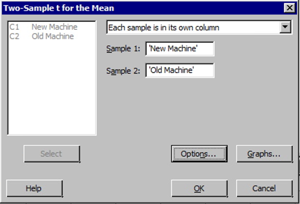
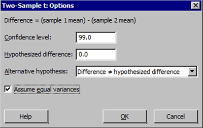 Note! When entering values into the samples in different columns input boxes, Minitab always subtracts the second value (column entered second) from the first value (column entered first).
 - Select the Options button and enter the desired 'confidence level', 'null hypothesis value' (again for our class this will be 0), and select the correct 'alternative hypothesis' from the drop-down menu. Finally, check the box for 'assume equal variances'. This latter selection should only be done when we have verified the two variances can be assumed equal.
The Minitab output for the packing time example:
Two-Sample T-Test and CI: New Machine, Old Machine
Method
μ1: mean of New Machine
μ2: mean of Old Machine
Difference: μ1 - μ2
Equal variances are assumed for this analysis.
Descriptive Statistics
| Sample |
N |
Mean |
StDev |
SE Mean |
|
New Machine |
10 |
42.140 |
0.683 | 0.22 |
|
Old Machine |
10 |
43.230 |
0.750 | 0.24 |
Estimation for Difference
| Difference | Pooled StDev | 95% Upper Bound for Difference |
|
-1.090 |
0.717 | -0.534 |
Test
Alternative hypothesis
H1: μ1 - μ2 < 0
| T-Value | DF | P-Value |
|---|---|---|
| -3.40 | 18 | 0.002 |
7.3.1.2 - Unpooled Variances
7.3.1.2 - Unpooled VariancesWhen the assumption of equal variances is not valid, we need to use separate, or unpooled, variances. The mathematics and theory are complicated for this case and we intentionally leave out the details.
We still have the following assumptions:
- The populations are independent
- Each population is either normal or the sample size is large.
If the assumptions are satisfied, then
\(t^*=\dfrac{\bar{x}_1-\bar{x_2}-0}{\sqrt{\frac{s^2_1}{n_1}+\frac{s^2_2}{n_2}}}\)
will have a t-distribution with degrees of freedom
\(df=\dfrac{(n_1-1)(n_2-1)}{(n_2-1)C^2+(1-C)^2(n_1-1)}\)
where \(C=\dfrac{\frac{s^2_1}{n_1}}{\frac{s^2_1}{n_1}+\frac{s^2_2}{n_2}}\).
- \((1-\alpha)100\%\) Confidence Interval for \(\mu_1-\mu_2\) for Unpooled Variances
- \(\bar{x}_1-\bar{x}_2\pm t_{\alpha/2} \sqrt{\frac{s^2_1}{n_1}+\frac{s^2_2}{n_2}}\)
-
Where \(t_{\alpha/2}\) comes from the t-distribution using the degrees of freedom above.
Minitab®
Minitab: Unpooled t-test
To perform a separate variance 2-sample, t-procedure use the same commands as for the pooled procedure EXCEPT we do NOT check box for 'Use Equal Variances.'
- Choose Stat > Basic Statistics > 2-sample t
- Select the Options box and enter the desired 'Confidence level,' 'Null hypothesis value' (again for our class this will be 0), and select the correct 'Alternative hypothesis' from the drop-down menu.
- Choose OK.
For some examples, one can use both the pooled t-procedure and the separate variances (non-pooled) t-procedure and obtain results that are close to each other. However, when the sample standard deviations are very different from each other, and the sample sizes are different, the separate variances 2-sample t-procedure is more reliable.
Example 7-5: Grade Point Average
Independent random samples of 17 sophomores and 13 juniors attending a large university yield the following data on grade point averages (student_gpa.txt):
| 3.04 | 2.92 | 2.86 | 1.71 | 3.60 |
| 3.49 | 3.30 | 2.28 | 3.11 | 2.88 |
| 2.82 | 2.13 | 2.11 | 3.03 | 3.27 |
| 2.60 | 3.13 |
| 2.56 | 3.47 | 2.65 | 2.77 | 3.26 |
| 3.00 | 2.70 | 3.20 | 3.39 | 3.00 |
| 3.19 | 2.58 | 2.98 |
At the 5% significance level, do the data provide sufficient evidence to conclude that the mean GPAs of sophomores and juniors at the university differ?
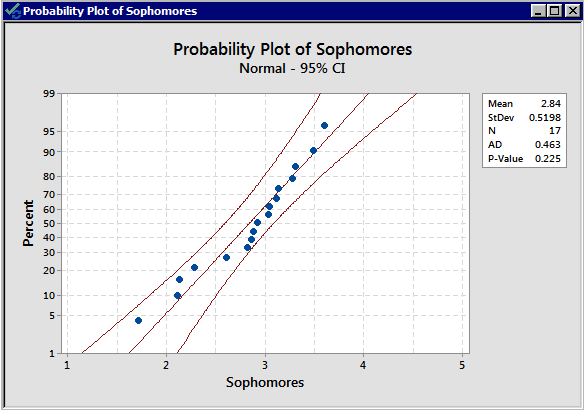
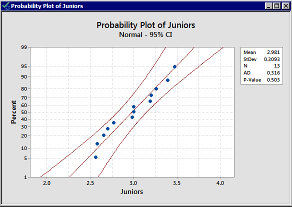
There is no indication that there is a violation of the normal assumption for both samples. As before, we should proceed with caution.
Now, we need to determine whether to use the pooled t-test or the non-pooled (separate variances) t-test. The summary statistics are:
|
Variable |
Sample size |
Mean |
Standard Deviation |
|---|---|---|---|
| sophomore |
17 |
2.840 |
0.52 |
|
junior |
13 |
2.981 |
0.3093 |
The standard deviations are 0.520 and 0.3093 respectively; both the sample sizes are small, and the standard deviations are quite different from each other. We, therefore, decide to use an unpooled t-test.
The null and alternative hypotheses are:
\(H_0\colon \mu_1-\mu_2=0\) vs \(H_a\colon \mu_1-\mu_2\ne0\)
The significance level is 5%. Perform the 2-sample t-test in Minitab with the appropriate alternative hypothesis.
Remember, the default for the 2-sample t-test in Minitab is the non-pooled one. Minitab generates the following output.
Two sample T for sophomores vs juniors
| N | Mean | StDev | SE Mean | |
|---|---|---|---|---|
| sophomore | 17 | 2.840 | 0.52 | 0.13 |
| junior | 13 | 2.981 | 0.309 | 0.086 |
95% CI for mu sophomore - mu juniors: (-0.45, 0.173)
T-Test mu sophomore = mu juniors (Vs no =): T = -0.92
P = 0.36 DF = 26
Since the p-value of 0.36 is larger than \(\alpha=0.05\), we fail to reject the null hypothesis.
At 5% level of significance, the data does not provide sufficient evidence that the mean GPAs of sophomores and juniors at the university are different.
95% CI for mu sophomore- mu juniors is;
(-0.45, 0.173)
We are 95% confident that the difference between the mean GPA of sophomores and juniors is between -0.45 and 0.173.
7.3.2 - Inference for Paired Means
7.3.2 - Inference for Paired MeansIntroduction
When we developed the inference for the independent samples, we depended on the statistical theory to help us. The theory, however, required the samples to be independent. What can we do when the two samples are not independent, i.e., the data is paired?
Consider an example where we are interested in a person’s weight before implementing a diet plan and after. Since the interest is focusing on the difference, it makes sense to “condense” these two measurements into one and consider the difference between the two measurements. For example, if instead of considering the two measures, we take the before diet weight and subtract the after diet weight. The difference makes sense too! It is the weight lost on the diet.
When we take the two measurements to make one measurement (i.e., the difference), we are now back to the one sample case! Now we can apply all we learned for the one sample mean to the difference (Cool!)
The Confidence Interval for the Difference of Paired Means, \(\mu_d\)
When we consider the difference of two measurements, the parameter of interest is the mean difference, denoted \(\mu_d\). The mean difference is the mean of the differences. We are still interested in comparing this difference to zero.
Suppose we have two paired samples of size \(n\):
\(x_1, x_2, …., x_n\) and \(y_1, y_2, … , y_n\)
Their difference can be denoted as:
\(d_1=x_1-y_1, d_2=x_2-y_2, …., d_n=x_n-y_n\)
The sample mean of the differences is:
\(\bar{d}=\frac{1}{n}\sum_{i=1}^n d_i\)
Denote the sample standard deviation of the differences as \(s_d\).
If \(\bar{d}\) is normal (or the sample size is large), the sampling distribution of \(\bar{d}\) is (approximately) normal with mean \(\mu_d\), standard error \(\dfrac{\sigma_d}{\sqrt{n}}\), and estimated standard error \(\dfrac{s_d}{\sqrt{n}}\).
At this point, the confidence interval will be the same as that of one sample.
- \(\boldsymbol{(1-\alpha)100\%}\) Confidence interval for \(\boldsymbol{\mu_d}\)
-
\(\bar{d}\pm t_{\alpha/2}\frac{s_d}{\sqrt{n}}\)
where \(t_{\alpha/2}\) comes from \(t\)-distribution with \(n-1\) degrees of freedom
Example 7-6: Zinc Concentrations
Trace metals in drinking water affect the flavor and an unusually high concentration can pose a health hazard. Ten pairs of data were taken measuring zinc concentration in bottom water and surface water (zinc_conc.txt).
Does the data suggest that the true average concentration in the bottom water is different than that of surface water? Construct a confidence interval to address this question.
Zinc concentrations
| 1 | 2 | 3 | 4 | 5 | 6 | 7 | 8 | 9 | 10 | |
|---|---|---|---|---|---|---|---|---|---|---|
| Bottom Water | .430 | .266 | .567 | .531 | .707 | .716 | .651 | .589 | .469 | .723 |
| Surface Water | .415 | .238 | .390 | .410 | .605 | .609 | .632 | .523 | .411 | .612 |
In this example, the response variable is concentration and is a quantitative measurement. The explanatory variable is location (bottom or surface) and is categorical. The two populations (bottom or surface) are not independent. Therefore, we are in the paired data setting. The parameter of interest is \(\mu_d\).
Find the difference as the concentration of the bottom water minus the concentration of the surface water.
Since the problem did not provide a confidence level, we should use 5%.
To use the methods we developed previously, we need to check the conditions. The problem does not indicate that the differences come from a normal distribution and the sample size is small (n=10). We should check, using the Normal Probability Plot to see if there is any violation. First, we need to find the differences.
|
Difference |
0.015 |
0.028 |
0.177 |
0.121 |
0.102 |
0.107 |
0.019 |
0.066 |
0.058 |
0.111 |
|---|
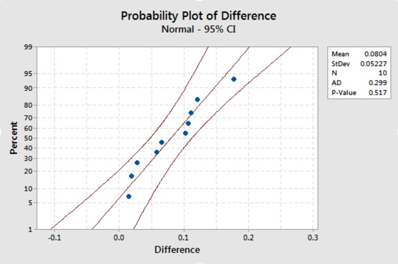
All of the differences fall within the boundaries, so there is no clear violation of the assumption. We can proceed with using our tools, but we should proceed with caution.
We need all of the pieces for the confidence interval. The sample mean difference is \(\bar{d}=0.0804\) and the standard deviation is \(s_d=0.0523\). For practice, you should find the sample mean of the differences and the standard deviation by hand. With \(n-1=10-1=9\) degrees of freedom, \(t_{0.05/2}=2.2622\).
The 95% confidence interval for the mean difference, \(\mu_d\) is:
\(\bar{d}\pm t_{\alpha/2}\dfrac{s_d}{\sqrt{n}}\)
\(0.0804\pm 2.2622\left( \dfrac{0.0523}{\sqrt{10}}\right)\)
(0.04299, 0.11781)
We are 95% confident that the population mean difference of bottom water and surface water zinc concentration is between 0.04299 and 0.11781.
If there is no difference between the means of the two measures, then the mean difference will be 0. Since 0 is not in our confidence interval, then the means are statistically different (or statistical significant or statistically different).
Note! Minitab will calculate the confidence interval and a hypothesis test simultaneously. We demonstrate how to find this interval using Minitab after presenting the hypothesis test.
Hypothesis Test for the Difference of Paired Means, \(\mu_d\)
In this section, we will develop the hypothesis test for the mean difference for paired samples. As we learned in the previous section, if we consider the difference rather than the two samples, then we are back in the one-sample mean scenario.
The possible null and alternative hypotheses are:
\(H_0\colon \mu_d=0\)
\(H_a\colon \mu_d\ne 0\)
\(H_a\colon \mu_d>0\)
\(H_a\colon \mu_d<0\)
We still need to check the conditions and at least one of the following need to be satisfied:
- The differences of the paired follow a normal distribution
- The sample size is large, \(n>30\).
If at least one is satisfied then...
\(t^*=\dfrac{\bar{d}-0}{\frac{s_d}{\sqrt{n}}}\)
Will follow a t-distribution with \(n-1\) degrees of freedom.
The same process for the hypothesis test for one mean can be applied. The test for the mean difference may be referred to as the paired t-test or the test for paired means.
Example 7-7: Zinc Concentrations - Hypothesis Test
Recall the zinc concentration example. Does the data suggest that the true average concentration in the bottom water exceeds that of surface water? Conduct this test using the rejection region approach. (zinc_conc.txt).
Zinc concentrations
| 1 | 2 | 3 | 4 | 5 | 6 | 7 | 8 | 9 | 10 | |
|---|---|---|---|---|---|---|---|---|---|---|
| Bottom Water | .430 | .266 | .567 | .531 | .707 | .716 | .651 | .589 | .469 | .723 |
| Surface Water | .415 | .238 | .390 | .410 | .605 | .609 | .632 | .523 | .411 | .612 |
If we find the difference as the concentration of the bottom water minus the concentration of the surface water, then null and alternative hypotheses are:
\(H_0\colon \mu_d=0\) vs \(H_a\colon \mu_d>0\)
Note! If the difference was defined as surface - bottom, then the alternative would be left-tailed.
The desired significance level was not stated so we will use \(\alpha=0.05\).
The assumptions were discussed when we constructed the confidence interval for this example. Remember although the Normal Probability Plot for the differences showed no violation, we should still proceed with caution.
The next step is to find the critical value and the rejection region. The critical value is the value \(a\) such that \(P(T>a)=0.05\). Using the table or software, the value is 1.8331. For a right-tailed test, the rejection region is \(t^*>1.8331\).
Recall from the previous example, the sample mean difference is \(\bar{d}=0.0804\) and the sample standard deviation of the difference is \(s_d=0.0523\). Therefore, the test statistic is:
\(t^*=\dfrac{\bar{d}-0}{\frac{s_d}{\sqrt{n}}}=\dfrac{0.0804}{\frac{0.0523}{\sqrt{10}}}=4.86\)
The value of our test statistic falls in the rejection region. Therefore, we reject the null hypothesis. With a significance level of 5%, there is enough evidence in the data to suggest that the bottom water has higher concentrations of zinc than the surface level.
Minitab® – Paired t-Test
You can use a paired t-test in Minitab to perform the test. Alternatively, you can perform a 1-sample t-test on difference = bottom - surface.
- Choose Stat> Basic Statistics> Paired t
- Click Optionsto specify the confidence level for the interval and the alternative hypothesis you want to test. The default null hypothesis is 0.
Zinc Concentrations Example
The Minitab output for paired T for bottom - surface is as follows:
Paired T for bottom - surface
|
N |
Mean |
StDev |
SE Mean |
|
|
bottom |
10 |
0.5649 |
0.1468 |
0.0464 |
|
surface |
10 |
0.4845 |
0.1312 |
0.0415 |
|
Difference |
10 |
0.0804 |
0.0523 |
0.0165 |
95% lower bound for mean difference: 0.0505
T-Test of mean difference = 0 (vs > 0): T-Value = 4.86 P-Value = 0.000
Note! In Minitab, if you choose a lower-tailed or an upper-tailed hypothesis test, an upper or lower confidence bound will be constructed, respectively, rather than a confidence interval.
Using the p-value to draw a conclusion about our example:
p-value = 0.000 < 0.05
Reject \(H_0\) and conclude that bottom zinc concentration is higher than surface zinc concentration.
Additional Notes
- For the zinc concentration problem, if you do not recognize the paired structure, but mistakenly use the 2-sample t-test treating them as independent samples, you will not be able to reject the null hypothesis. This demonstrates the importance of distinguishing the two types of samples. Also, it is wise to design an experiment efficiently whenever possible.
- What if the assumption of normality is not satisfied? Considering a nonparametric test would be wise.
7.4 - Comparing Two Population Variances
7.4 - Comparing Two Population VariancesSo far, we considered inference to compare two proportions and inference to compare two means. In this section, we will present how to compare two population variances.
Why would we want to compare two population variances? There are many situations, such as in quality control problems, where you may want to choose the process with smaller variability for a variable of interest.
One of the essential steps of a test to compare two population variances is for checking the equal variances assumption if you want to use the pooled variances. Many people use this test as a guide to see if there are any clear violations, much like using the rule of thumb.
When we introduce inference for two parameters before, we started with the sampling distribution. We will not do this here. The details of this test are left out. We will simply present how to use it.
F-Test to Compare Two Population Variances
To compare the variances of two quantitative variables, the hypotheses of interest are:
\(H_0\colon \dfrac{\sigma^2_1}{\sigma^2_2}=1\)
\(H_a\colon \dfrac{\sigma^2_1}{\sigma^2_2}\ne1\)
\(H_a\colon \dfrac{\sigma^2_1}{\sigma^2_2}>1\)
\(H_a\colon \dfrac{\sigma^2_1}{\sigma^2_2}<1\)
The last two alternatives are determined by how you arrange your ratio of the two sample statistics.
We will rely on Minitab to conduct this test for us. Minitab offers three (3) different methods to test equal variances.
- The F-test: This test assumes the two samples come from populations that are normally distributed.
- Bonett's test: this assumes only that the two samples are quantitative.
- Levene's test: similar to Bonett's in that the only assumption is that the data is quantitative. Best to use if one or both samples are heavily skewed, and your two sample sizes are both under 20.
Bonett’s test and Levene’s test are both considered nonparametric tests. In our case, since the tests we will be considering are based on a normal distribution, we are expecting to use the F-test. Again, we will need to confirm this by plotting our sample data (i.e., using a probability plot).
Caution! To use the F-test, the samples must come from a normal distribution. The Central Limit Theorem applies to sample means, not to the data. Therefore, if the sample size is large, it does not mean we can assume the data come from a normal distribution.
Example 7-8: Comparing Packing Time Variances
Using the data in the packaging time from our previous discussion on two independent samples, we want to check whether it is reasonable to assume that the two machines have equal population variances.
Recall that the data are given below as (machine.txt):
-
42.1 41.3 42.4 43.2 41.8 41.0 41.8 42.8 42.3 42.7 - \(\bar{x}_1=42.14, \text{s}_1= 0.683\)
-
42.7 43.8 42.5 43.1 44.0 43.6 43.3 43.5 41.7 44.1 - \(\bar{x}_2=43.23, \text{s}_2= 0.750\)
Minitab: F-test to Compare Two Population Variances
In Minitab...
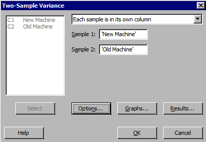
- Choose Stat > Basic Statistics > 2 Variances and complete the dialog boxes.
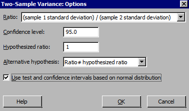
- In the dialog box, check 'Use test and confidence intervals based on normal distribution' when we are confident the two samples come from a normal distribution.
Notes on using Minitab:
- Minitab will compare the two variances using the popular F-test method.
- If we only have summarized data (e.g. the sample sizes and sample variances or sample standard deviations), then the two variance test in Minitab will only provide an F-test.
- Minitab will use the Bonett and Levene test that are more robust tests when normality is not assumed.
- Minitab calculates the ratio based on Sample 1 divided by Sample 2.
The Minitab Output for the test for equal variances is as follows (a graph is also given in the output that provides confidence intervals and p-value for the test. This is not shown here):
Test and CI for Two Variances: New machine, Old machine
Method
σ1: standard deviation of New machine
σ2: standard deviation of Old machine
Ratio: σ1/σ2
F method was used. This method is accurate for normal data only.
Descriptive Statistics
| Variable | N | StDev | Variance | 95% CI for σ |
|---|---|---|---|---|
| New Machine | 10 | 0.683 | 0.467 | (0.470, 1.248) |
| Old Machine | 10 | 0.750 | 0.562 | (0.516, 1.369) |
Ratio of standard deviations
| Estimated Ratio | 95% CI for Ratio using F |
|---|---|
| 0.911409 | (0454, 1.829) |
Tests
Null hypothesis
Alternative hypothesis
Significance level
H0: σ1/σ2=1
H1: σ1/σ2≠1
α=0.05
| Method | Test Statistic | DF1 | DF2 | P-Value |
|---|---|---|---|---|
| F | 0.83 | 9 | 9 | 0.787 |
How do we interpret the Minitab output?
Note that \(S_{new}=0.683\) and \(s_{old}=0.750\) The test statistic \(F\) is computed as...
\(F=\dfrac{s^2_{new}}{s^2_{old}}=0.83\)
The p-value provided is that for the alternative selected i.e. two-sided. If the alternative were one sided, for example if our alternative in the above example was "ratio less than 1", then the p-value would be half the reported p-value for the two-sided test, or 0.393.
Minitab provided the results only from the F-test since we checked the box to assume normal distribution. Regardless, the hypotheses would be the same for any of the test options and the decision method is the same: if the p-value is less than alpha, we reject the null and conclude the two population variances are not equal. Otherwise, if the p-value is large (i.e. greater than alpha) then we fail to reject the null and can assume the two population variances are equal.
In this example, the p-value for the F-test is very large (larger than 0.1). Therefore, we fail to reject the null hypothesis and conclude that there is not enough evidence to conclude the variances are different.
Note! Remember, if there is doubt about normality, the better choice is to NOT use the F-test. You need to check whether the normal assumption holds before you can use the F-test since the F-test is very sensitive to departure from the normal assumption.
7.5 - Lesson 7 Summary
7.5 - Lesson 7 SummaryIn this Lesson, we discussed how to compare population parameters from two samples. It is important to recognize which parameters are of interest. Once we identify the parameters, there are different approaches based on what we can assume about the samples.
We compared two population proportions for independent samples by developing the confidence interval and the hypothesis test for the difference between the two population proportions.
Next, we discussed how to compare two population means. The approach for inference is different if the samples are paired or independent. For two independent samples, we presented two cases based on whether or not we can assume the population variances are the same.
Finally, we discussed a test for comparing two sample variances from independent samples using the F-test.
In this Lesson, we considered the cases where the response is either qualitative or quantitative, and the explanatory variable is qualitative (categorical). In the next Lesson, we will present the case where both the response and the explanatory variable are qualitative.