7.3.1 - Inference for Independent Means
7.3.1 - Inference for Independent MeansTwo-Cases for Independent Means
As with comparing two population proportions, when we compare two population means from independent populations, the interest is in the difference of the two means. In other words, if \(\mu_1\) is the population mean from population 1 and \(\mu_2\) is the population mean from population 2, then the difference is \(\mu_1-\mu_2\). If \(\mu_1-\mu_2=0\) then there is no difference between the two population parameters.
If each population is normal, then the sampling distribution of \(\bar{x}_i\) is normal with mean \(\mu_i\), standard error \(\dfrac{\sigma_i}{\sqrt{n_i}}\), and the estimated standard error \(\dfrac{s_i}{\sqrt{n_i}}\), for \(i=1, 2\).
Using the Central Limit Theorem, if the population is not normal, then with a large sample, the sampling distribution is approximately normal.
The theorem presented in this Lesson says that if either of the above are true, then \(\bar{x}_1-\bar{x}_2\) is approximately normal with mean \(\mu_1-\mu_2\), and standard error \(\sqrt{\dfrac{\sigma^2_1}{n_1}+\dfrac{\sigma^2_2}{n_2}}\).
However, in most cases, \(\sigma_1\) and \(\sigma_2\) are unknown, and they have to be estimated. It seems natural to estimate \(\sigma_1\) by \(s_1\) and \(\sigma_2\) by \(s_2\). When the sample sizes are small, the estimates may not be that accurate and one may get a better estimate for the common standard deviation by pooling the data from both populations if the standard deviations for the two populations are not that different.
Given this, there are two options for estimating the variances for the independent samples:
- Using pooled variances
- Using unpooled (or unequal) variances
When to use which? When we are reasonably sure that the two populations have nearly equal variances, then we use the pooled variances test. Otherwise, we use the unpooled (or separate) variance test.
7.3.1.1 - Pooled Variances
7.3.1.1 - Pooled VariancesConfidence Intervals for \(\boldsymbol{\mu_1-\mu_2}\): Pooled Variances
When we have good reason to believe that the variance for population 1 is equal to that of population 2, we can estimate the common variance by pooling information from samples from population 1 and population 2.
An informal check for this is to compare the ratio of the two sample standard deviations. If the two are equal, the ratio would be 1, i.e. \(\frac{s_1}{s_2}=1\). However, since these are samples and therefore involve error, we cannot expect the ratio to be exactly 1. When the sample sizes are nearly equal (admittedly "nearly equal" is somewhat ambiguous, so often if sample sizes are small one requires they be equal), then a good Rule of Thumb to use is to see if the ratio falls from 0.5 to 2. That is, neither sample standard deviation is more than twice the other.
If this rule of thumb is satisfied, we can assume the variances are equal. Later in this lesson, we will examine a more formal test for equality of variances.
- Let \(n_1\) be the sample size from population 1 and let \(s_1\) be the sample standard deviation of population 1.
- Let \(n_2\) be the sample size from population 2 and \(s_2\) be the sample standard deviation of population 2.
Then the common standard deviation can be estimated by the pooled standard deviation:
\(s_p=\sqrt{\dfrac{(n_1-1)s_1^2+(n_2-1)s^2_2}{n_1+n_2-2}}\)
If we can assume the populations are independent, that each population is normal or has a large sample size, and that the population variances are the same, then it can be shown that...
\(t=\dfrac{\bar{x}_1-\bar{x_2}-0}{s_p\sqrt{\frac{1}{n_1}+\frac{1}{n_2}}}\)
follows a t-distribution with \(n_1+n_2-2\) degrees of freedom.
Now, we can construct a confidence interval for the difference of two means, \(\mu_1-\mu_2\).
- \(\boldsymbol{(1-\alpha)100\%}\) Confidence interval for \(\boldsymbol{\mu_1-\mu_2}\) for Pooled Variances
- \(\bar{x}_1-\bar{x}_2\pm t_{\alpha/2}s_p\sqrt{\frac{1}{n_1}+\frac{1}{n_2}}\)
-
where \(t_{\alpha/2}\) comes from a t-distribution with \(n_1+n_2-2\) degrees of freedom.
Hypothesis Tests for \(\boldsymbol{\mu_1-\mu_2}\): The Pooled t-test
Now let's consider the hypothesis test for the mean differences with pooled variances.
\(H_0\colon\mu_1-\mu_2=0\)
\(H_a\colon \mu_1-\mu_2\ne0\)
\(H_a\colon \mu_1-\mu_2>0\)
\(H_a\colon \mu_1-\mu_2<0\)
The assumptions/conditions are:
- The populations are independent
- The population variances are equal
- Each population is either normal or the sample size is large.
The test statistic is...
\(t^*=\dfrac{\bar{x}_1-\bar{x}_2-0}{s_p\sqrt{\frac{1}{n_1}+\frac{1}{n_2}}}\)
And \(t^*\) follows a t-distribution with degrees of freedom equal to \(df=n_1+n_2-2\).
The p-value, critical value, rejection region, and conclusion are found similarly to what we have done before.
Example 7-4: Comparing Packing Machines
In a packing plant, a machine packs cartons with jars. It is supposed that a new machine will pack faster on the average than the machine currently used. To test that hypothesis, the times it takes each machine to pack ten cartons are recorded. The results, (machine.txt), in seconds, are shown in the tables.
| 42.1 | 41.3 | 42.4 | 43.2 | 41.8 |
| 41.0 | 41.8 | 42.8 | 42.3 | 42.7 |
\(\bar{x}_1=42.14, \text{s}_1= 0.683\)
| 42.7 | 43.8 | 42.5 | 43.1 | 44.0 |
| 43.6 | 43.3 | 43.5 | 41.7 | 44.1 |
\(\bar{x}_2=43.23, \text{s}_2= 0.750\)
Do the data provide sufficient evidence to conclude that, on the average, the new machine packs faster?
Are these independent samples? Yes, since the samples from the two machines are not related.
Are these large samples or a normal population?
We have \(n_1\lt 30\) and \(n_2\lt 30\). We do not have large enough samples, and thus we need to check the normality assumption from both populations. Let's take a look at the normality plots for this data:
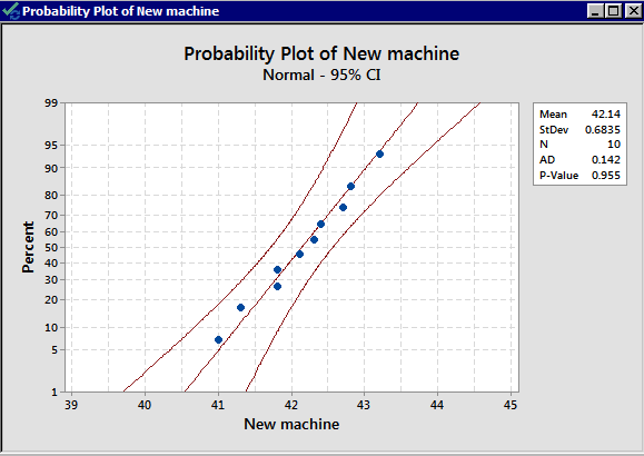
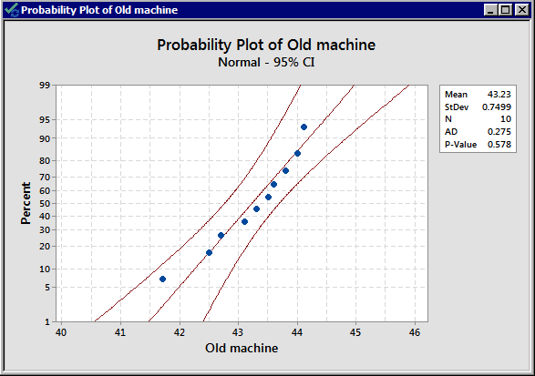
From the normal probability plots, we conclude that both populations may come from normal distributions. Remember the plots do not indicate that they DO come from a normal distribution. It only shows if there are clear violations. We should proceed with caution.
Do the populations have equal variance? No information allows us to assume they are equal. We can use our rule of thumb to see if they are “close.” They are not that different as \(\dfrac{s_1}{s_2}=\dfrac{0.683}{0.750}=0.91\) is quite close to 1. This assumption does not seem to be violated.
We can thus proceed with the pooled t-test.
Let \(\mu_1\) denote the mean for the new machine and \(\mu_2\) denote the mean for the old machine.
The null hypothesis is that there is no difference in the two population means, i.e.
\(H_0\colon \mu_1-\mu_2=0\)
The alternative is that the new machine is faster, i.e.
\(H_a\colon \mu_1-\mu_2<0\)
The significance level is 5%. Since we may assume the population variances are equal, we first have to calculate the pooled standard deviation:
\begin{align} s_p&=\sqrt{\frac{(n_1-1)s^2_1+(n_2-1)s^2_2}{n_1+n_2-2}}\\ &=\sqrt{\frac{(10-1)(0.683)^2+(10-1)(0.750)^2}{10+10-2}}\\ &=\sqrt{\dfrac{9.261}{18}}\\ &=0.7173 \end{align}
The test statistic is:
\begin{align} t^*&=\dfrac{\bar{x}_1-\bar{x}_2-0}{s_p\sqrt{\frac{1}{n_1}+\frac{1}{n_2}}}\\ &=\dfrac{42.14-43.23}{0.7173\sqrt{\frac{1}{10}+\frac{1}{10}}}\\&=-3.398 \end{align}
The alternative is left-tailed so the critical value is the value \(a\) such that \(P(T<a)=0.05\), with \(10+10-2=18\) degrees of freedom. The critical value is -1.7341. The rejection region is \(t^*<-1.7341\).
Our test statistic, -3.3978, is in our rejection region, therefore, we reject the null hypothesis. With a significance level of 5%, we reject the null hypothesis and conclude there is enough evidence to suggest that the new machine is faster than the old machine.
To find the interval, we need all of the pieces. We calculated all but one when we conducted the hypothesis test. We only need the multiplier. For a 99% confidence interval, the multiplier is \(t_{0.01/2}\) with degrees of freedom equal to 18. This value is 2.878.
The interval is:
\(\bar{x}_1-\bar{x}_2\pm t_{\alpha/2}s_p\sqrt{\frac{1}{n_1}+\frac{1}{n_2}}\)
\((42.14-43.23)\pm 2.878(0.7173)\sqrt{\frac{1}{10}+\frac{1}{10}}\)
\(-1.09\pm 0.9232\)
The 99% confidence interval is (-2.013, -0.167).
We are 99% confident that the difference between the two population mean times is between -2.012 and -0.167.
Minitab: 2-Sample t-test - Pooled
The following steps are used to conduct a 2-sample t-test for pooled variances in Minitab.
- Choose Stat > Basic Statistics > 2-Sample t .
- The following dialog boxes will then be displayed.
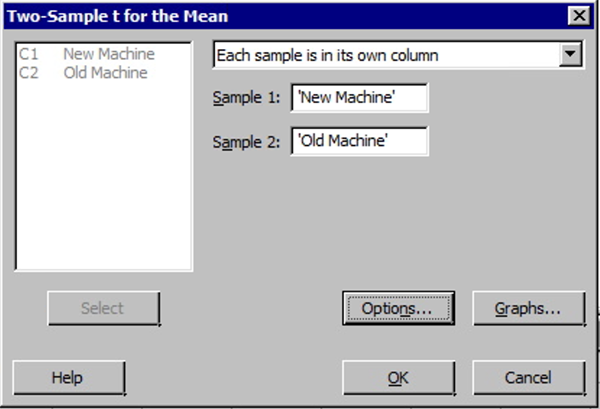
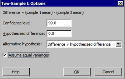 Note! When entering values into the samples in different columns input boxes, Minitab always subtracts the second value (column entered second) from the first value (column entered first).
 - Select the Options button and enter the desired 'confidence level', 'null hypothesis value' (again for our class this will be 0), and select the correct 'alternative hypothesis' from the drop-down menu. Finally, check the box for 'assume equal variances'. This latter selection should only be done when we have verified the two variances can be assumed equal.
The Minitab output for the packing time example:
Two-Sample T-Test and CI: New Machine, Old Machine
Method
μ1: mean of New Machine
μ2: mean of Old Machine
Difference: μ1 - μ2
Equal variances are assumed for this analysis.
Descriptive Statistics
| Sample |
N |
Mean |
StDev |
SE Mean |
|
New Machine |
10 |
42.140 |
0.683 | 0.22 |
|
Old Machine |
10 |
43.230 |
0.750 | 0.24 |
Estimation for Difference
| Difference | Pooled StDev | 95% Upper Bound for Difference |
|
-1.090 |
0.717 | -0.534 |
Test
Alternative hypothesis
H1: μ1 - μ2 < 0
| T-Value | DF | P-Value |
|---|---|---|
| -3.40 | 18 | 0.002 |
7.3.1.2 - Unpooled Variances
7.3.1.2 - Unpooled VariancesWhen the assumption of equal variances is not valid, we need to use separate, or unpooled, variances. The mathematics and theory are complicated for this case and we intentionally leave out the details.
We still have the following assumptions:
- The populations are independent
- Each population is either normal or the sample size is large.
If the assumptions are satisfied, then
\(t^*=\dfrac{\bar{x}_1-\bar{x_2}-0}{\sqrt{\frac{s^2_1}{n_1}+\frac{s^2_2}{n_2}}}\)
will have a t-distribution with degrees of freedom
\(df=\dfrac{(n_1-1)(n_2-1)}{(n_2-1)C^2+(1-C)^2(n_1-1)}\)
where \(C=\dfrac{\frac{s^2_1}{n_1}}{\frac{s^2_1}{n_1}+\frac{s^2_2}{n_2}}\).
- \((1-\alpha)100\%\) Confidence Interval for \(\mu_1-\mu_2\) for Unpooled Variances
- \(\bar{x}_1-\bar{x}_2\pm t_{\alpha/2} \sqrt{\frac{s^2_1}{n_1}+\frac{s^2_2}{n_2}}\)
-
Where \(t_{\alpha/2}\) comes from the t-distribution using the degrees of freedom above.
Minitab®
Minitab: Unpooled t-test
To perform a separate variance 2-sample, t-procedure use the same commands as for the pooled procedure EXCEPT we do NOT check box for 'Use Equal Variances.'
- Choose Stat > Basic Statistics > 2-sample t
- Select the Options box and enter the desired 'Confidence level,' 'Null hypothesis value' (again for our class this will be 0), and select the correct 'Alternative hypothesis' from the drop-down menu.
- Choose OK.
For some examples, one can use both the pooled t-procedure and the separate variances (non-pooled) t-procedure and obtain results that are close to each other. However, when the sample standard deviations are very different from each other, and the sample sizes are different, the separate variances 2-sample t-procedure is more reliable.
Example 7-5: Grade Point Average
Independent random samples of 17 sophomores and 13 juniors attending a large university yield the following data on grade point averages (student_gpa.txt):
| 3.04 | 2.92 | 2.86 | 1.71 | 3.60 |
| 3.49 | 3.30 | 2.28 | 3.11 | 2.88 |
| 2.82 | 2.13 | 2.11 | 3.03 | 3.27 |
| 2.60 | 3.13 |
| 2.56 | 3.47 | 2.65 | 2.77 | 3.26 |
| 3.00 | 2.70 | 3.20 | 3.39 | 3.00 |
| 3.19 | 2.58 | 2.98 |
At the 5% significance level, do the data provide sufficient evidence to conclude that the mean GPAs of sophomores and juniors at the university differ?
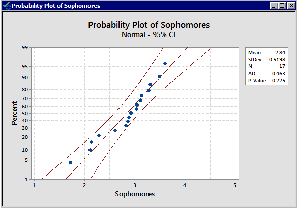
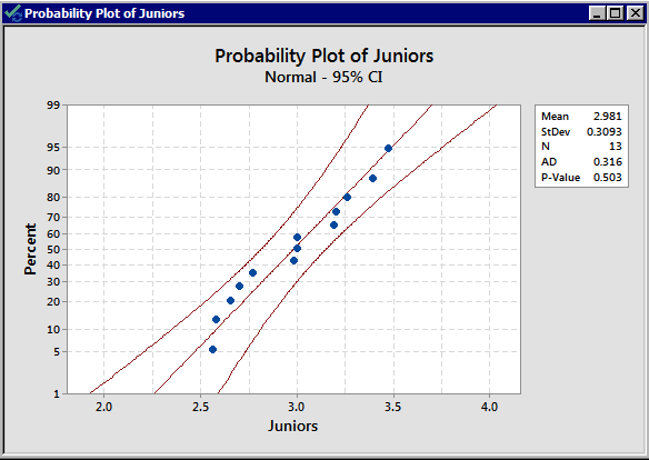
There is no indication that there is a violation of the normal assumption for both samples. As before, we should proceed with caution.
Now, we need to determine whether to use the pooled t-test or the non-pooled (separate variances) t-test. The summary statistics are:
|
Variable |
Sample size |
Mean |
Standard Deviation |
|---|---|---|---|
| sophomore |
17 |
2.840 |
0.52 |
|
junior |
13 |
2.981 |
0.3093 |
The standard deviations are 0.520 and 0.3093 respectively; both the sample sizes are small, and the standard deviations are quite different from each other. We, therefore, decide to use an unpooled t-test.
The null and alternative hypotheses are:
\(H_0\colon \mu_1-\mu_2=0\) vs \(H_a\colon \mu_1-\mu_2\ne0\)
The significance level is 5%. Perform the 2-sample t-test in Minitab with the appropriate alternative hypothesis.
Remember, the default for the 2-sample t-test in Minitab is the non-pooled one. Minitab generates the following output.
Two sample T for sophomores vs juniors
| N | Mean | StDev | SE Mean | |
|---|---|---|---|---|
| sophomore | 17 | 2.840 | 0.52 | 0.13 |
| junior | 13 | 2.981 | 0.309 | 0.086 |
95% CI for mu sophomore - mu juniors: (-0.45, 0.173)
T-Test mu sophomore = mu juniors (Vs no =): T = -0.92
P = 0.36 DF = 26
Since the p-value of 0.36 is larger than \(\alpha=0.05\), we fail to reject the null hypothesis.
At 5% level of significance, the data does not provide sufficient evidence that the mean GPAs of sophomores and juniors at the university are different.
95% CI for mu sophomore- mu juniors is;
(-0.45, 0.173)
We are 95% confident that the difference between the mean GPA of sophomores and juniors is between -0.45 and 0.173.