7.3.1.2 - Unpooled Variances
7.3.1.2 - Unpooled VariancesWhen the assumption of equal variances is not valid, we need to use separate, or unpooled, variances. The mathematics and theory are complicated for this case and we intentionally leave out the details.
We still have the following assumptions:
- The populations are independent
- Each population is either normal or the sample size is large.
If the assumptions are satisfied, then
\(t^*=\dfrac{\bar{x}_1-\bar{x_2}-0}{\sqrt{\frac{s^2_1}{n_1}+\frac{s^2_2}{n_2}}}\)
will have a t-distribution with degrees of freedom
\(df=\dfrac{(n_1-1)(n_2-1)}{(n_2-1)C^2+(1-C)^2(n_1-1)}\)
where \(C=\dfrac{\frac{s^2_1}{n_1}}{\frac{s^2_1}{n_1}+\frac{s^2_2}{n_2}}\).
- \((1-\alpha)100\%\) Confidence Interval for \(\mu_1-\mu_2\) for Unpooled Variances
- \(\bar{x}_1-\bar{x}_2\pm t_{\alpha/2} \sqrt{\frac{s^2_1}{n_1}+\frac{s^2_2}{n_2}}\)
-
Where \(t_{\alpha/2}\) comes from the t-distribution using the degrees of freedom above.
Minitab®
Minitab: Unpooled t-test
To perform a separate variance 2-sample, t-procedure use the same commands as for the pooled procedure EXCEPT we do NOT check box for 'Use Equal Variances.'
- Choose Stat > Basic Statistics > 2-sample t
- Select the Options box and enter the desired 'Confidence level,' 'Null hypothesis value' (again for our class this will be 0), and select the correct 'Alternative hypothesis' from the drop-down menu.
- Choose OK.
For some examples, one can use both the pooled t-procedure and the separate variances (non-pooled) t-procedure and obtain results that are close to each other. However, when the sample standard deviations are very different from each other, and the sample sizes are different, the separate variances 2-sample t-procedure is more reliable.
Example 7-5: Grade Point Average
Independent random samples of 17 sophomores and 13 juniors attending a large university yield the following data on grade point averages (student_gpa.txt):
| 3.04 | 2.92 | 2.86 | 1.71 | 3.60 |
| 3.49 | 3.30 | 2.28 | 3.11 | 2.88 |
| 2.82 | 2.13 | 2.11 | 3.03 | 3.27 |
| 2.60 | 3.13 |
| 2.56 | 3.47 | 2.65 | 2.77 | 3.26 |
| 3.00 | 2.70 | 3.20 | 3.39 | 3.00 |
| 3.19 | 2.58 | 2.98 |
At the 5% significance level, do the data provide sufficient evidence to conclude that the mean GPAs of sophomores and juniors at the university differ?
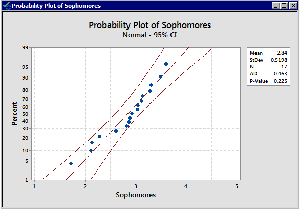
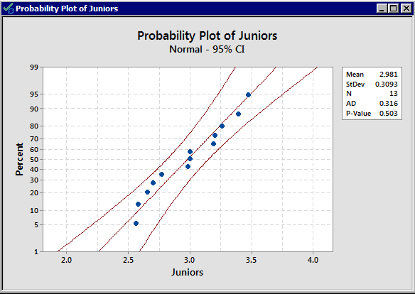
There is no indication that there is a violation of the normal assumption for both samples. As before, we should proceed with caution.
Now, we need to determine whether to use the pooled t-test or the non-pooled (separate variances) t-test. The summary statistics are:
|
Variable |
Sample size |
Mean |
Standard Deviation |
|---|---|---|---|
| sophomore |
17 |
2.840 |
0.52 |
|
junior |
13 |
2.981 |
0.3093 |
The standard deviations are 0.520 and 0.3093 respectively; both the sample sizes are small, and the standard deviations are quite different from each other. We, therefore, decide to use an unpooled t-test.
The null and alternative hypotheses are:
\(H_0\colon \mu_1-\mu_2=0\) vs \(H_a\colon \mu_1-\mu_2\ne0\)
The significance level is 5%. Perform the 2-sample t-test in Minitab with the appropriate alternative hypothesis.
Remember, the default for the 2-sample t-test in Minitab is the non-pooled one. Minitab generates the following output.
Two sample T for sophomores vs juniors
| N | Mean | StDev | SE Mean | |
|---|---|---|---|---|
| sophomore | 17 | 2.840 | 0.52 | 0.13 |
| junior | 13 | 2.981 | 0.309 | 0.086 |
95% CI for mu sophomore - mu juniors: (-0.45, 0.173)
T-Test mu sophomore = mu juniors (Vs no =): T = -0.92
P = 0.36 DF = 26
Since the p-value of 0.36 is larger than \(\alpha=0.05\), we fail to reject the null hypothesis.
At 5% level of significance, the data does not provide sufficient evidence that the mean GPAs of sophomores and juniors at the university are different.
95% CI for mu sophomore- mu juniors is;
(-0.45, 0.173)
We are 95% confident that the difference between the mean GPA of sophomores and juniors is between -0.45 and 0.173.