9.1 - Linear Relationships
9.1 - Linear RelationshipsTo define a useful model, we must investigate the relationship between the response and the predictor variables. As mentioned before, the focus of this Lesson is linear relationships.
For a brief review of linear functions, recall that the equation of a line has the following form:
\(y=mx+b\)
where m is the slope and b is the y-intercept.
Given two points on a line, \((x_1, y_1)\) and \((x_2, y_2)\), the slope is calculated by:
\begin{align} m&=\dfrac{y_2-y_1}{x_2-x_1}\\&=\dfrac{\text{change in y}}{\text{change in x}}\\&=\frac{\text{rise}}{\text{run}} \end{align}
The slope of a line describes a lot about the linear relationship between two variables. If the slope is positive, then there is a positive linear relationship, i.e., as one increases, the other increases. If the slope is negative, then there is a negative linear relationship, i.e., as one increases the other variable decreases. If the slope is 0, then as one increases, the other remains constant.
When we look for linear relationships between two variables, it is rarely the case where the coordinates fall exactly on a straight line; there will be some error. In the next sections, we will show how to examine the data for a linear relationship (i.e., the scatterplot) and how to find a measure to describe the linear relationship (i.e., correlation).
9.1.1 - Scatterplots
9.1.1 - ScatterplotsIf the interest is to investigate the relationship between two quantitative variables, one valuable tool is the scatterplot.
- Scatterplot
- A graphical representation of two quantitative variables where the explanatory variable is on the x-axis and the response variable is on the y-axis.
When we look at the scatterplot, keep in mind the following questions:
- What is the direction of the relationship?
- Is the relationship linear or nonlinear?
- Is the relationship weak, moderate, or strong?
- Are there any outliers or extreme values?
We describe the direction of the relationship as positive or negative. A positive relationship means that as the value of the explanatory variable increases, the value of the response variable increases, in general. A negative relationship implies that as the value of the explanatory variable increases, the value of the response variable tends to decrease.
Example 9-1: Student height and weight (Scatterplots)
Suppose we took a sample from students at a large university and asked them about their height and weight. The data can be found here university_ht_wt.txt.
The first three observations are:
|
Height (inches) |
Weight (pounds) |
|---|---|
|
72 |
200 |
|
68 |
165 |
|
69 |
160 |
We let \(X\) denote the height and \(Y\) denote the weight of the student. The observations are then considered as coordinates \((x,y)\). For example, student 1 has coordinate (72,200). These coordinates are plotted on the x-y plane.
We can use Minitab to create the scatterplot.
Minitab: Scatterplots
We can create our scatterplot in Minitab following these steps.
- Choose Graph > Scatterplot > Simple
- Choose OK
Scatterplot of Weight vs Height
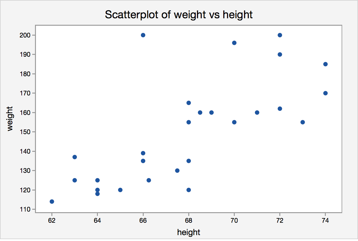
The scatterplot shows that, in general, as height increases, weight increases. We say “in general” because it is not always the case. For example, the observation with a height of 66 inches and a weight of 200 pounds does not seem to follow the trend of the data.
The two variables seem to have a positive relationship. As the height increases, weight tends to increase as well. The relationship does not seem to be perfectly linear, i.e., the points do not fall on a straight line, but it does seem to follow a straight line moderately, with some variability.
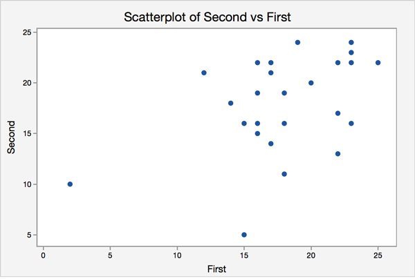
Try it!
An elementary school teacher gives her students two spelling tests a year. Each test contains 24 words, and the score is the number of words spelled correctly. The teacher is interested in the relationship between the score on the first test and the score on the second test. Using the scatterplot, comment on the relationship between the two variables.
In the next section, we will introduce correlation. Correlation is a measure that gives us an idea of the strength and direction of the linear relationship between two quantitative variables.
9.1.2 - Correlation
9.1.2 - CorrelationIf we want to provide a measure of the strength of the linear relationship between two quantitative variables, a good way is to report the correlation coefficient between them.
The sample correlation coefficient is typically denoted as \(r\). It is also known as Pearson’s \(r\). The population correlation coefficient is generally denoted as \(\rho\), pronounced “rho.”
- Sample Correlation Coefficient
-
The sample correlation coefficient, \(r\), is calculated using the following formula:
\( r=\dfrac{\sum (x_i-\bar{x})(y_i-\bar{y}) }{\sqrt{\sum (x_i-\bar{x})^2}\sqrt{\sum (y_i-\bar{y})^2}} \)
Properties of the correlation coefficient, \(r\):
- \(-1\le r\le 1\), i.e. \(r\) takes values between -1 and +1, inclusive.
- The sign of the correlation provides the direction of the linear relationship. The sign indicates whether the two variables are positively or negatively related.
- A correlation of 0 means there is no linear relationship.
- There are no units attached to \(r\).
- As the magnitude of \(r\) approaches 1, the stronger the linear relationship.
- As the magnitude of \(r \) approaches 0, the weaker the linear relationship.
- If we fit the simple linear regression model between Y and X, then \(r\) has the same sign as \(\beta_1\), which is the coefficient of X in the linear regression equation. -- more on this later.
- The correlation value would be the same regardless of which variable we defined as X and Y.
Note! The correlation is unit free. We can see this easier using the equation above. Consider, for example, that we are interested in the correlation between X = height (inches) and Y = weight (pounds). In the equation above, the numerator would have the units of \(\text{pounds}^*\text{inches}\). The denominator would include taking the square root of pounds squared and inches squared, leaving us again with units of \(\text{pounds}^*\text{inches}\). Therefore the units would cancel out.
Visualizing Correlation
The following four graphs illustrate four possible situations for the values of r. Pay particular attention to graph (d) which shows a strong relationship between y and x but where r = 0. Note that no linear relationship does not imply no relationship exists!
a) \(r > 0\)
b) \(r < 0\)
c) \(r = 0\)
d) \(r=0\)
Example 9-2: Sales and Advertising (Correlation)
We have collected five months of sales and advertising dollars for a small company we own. Sales units are in thousands of dollars, and advertising units are in hundreds of dollars. Our interest is determining if a linear relationship exists between sales and advertising. The data is as follows:
| Sales (Y) | Advertising (X) |
|---|---|
| 1 | 1 |
| 1 | 2 |
| 2 | 3 |
| 2 | 4 |
| 4 | 5 |
Find the sample correlation and interpret the value.
| \(y_i-\bar{y}\) | \(x_i-\bar{x}\) | \((x_i-\bar{x})(y_i-\bar{y})\) |
|---|---|---|
| \(1-2=-1\) | \(1-3=-2\) | \((-1)(-2)=2\) |
| \(1-2=-1\) | \(2-3=-1\) | \((-1)(-1)=1\) |
| \(2-2=0\) | \(3-3=0\) | \((0)(0)=0\) |
| \(2-2=0\) | \(4-3=1\) | \((0)(1)=0\) |
| \(4-2=2\) | \(5-3=2\) | \((2)(2)=4\) |
From the table we can calculate the following sums...
\(\sum(y_i-\bar{y})^2=(-1)^2+(-1)^2+0+0+2^2=6 \;\text{(sum of first column)}\)
\(\sum(x_i-\bar{x})^2=(-2)^2+(-1)^2+0+1^2+2^2=10 \;\text{(sum of second column)}\)
\(\sum(x_i-\bar{x})(y_i-\bar{y})=2+1+0+0+4=7 \;\text{(sum of third column)}\)
Using these numbers in the formula for r...
\(r=\dfrac{\sum (x_i-\bar{x})(y_i-\bar{y})}{\sqrt{\sum(x_i-\bar{x})^2}\sqrt{\sum(y_i-\bar{y})^2}}=\dfrac{7}{\sqrt{10}\sqrt{6}}=0.9037\)
Using Minitab to calculate r
To calculate r using Minitab:
- Open Minitab and upload the data (for this example type the Y data into a column (e.g., C1) and the X data into a column (e.g., C2))
- Choose Stat > Basic Statistics > Correlation
- Specify the response and explanatory variables in the dialog box (X and Y in this example).
Minitab output for this example:
Correlation: Y,X
Correlations
P-value
0.035
The sample correlation is 0.904. This value indicates a strong positive linear relationship between sales and advertising.
Try it!
Using the following data, calculate the correlation and interpret the value.
| X | Y |
|---|---|
| 2 | 7 |
| 4 | 11 |
| 14 | 29 |
| 13 | 28 |
| 15 | 32 |
The mean of \(X\) is 9.6 and the mean of \(Y\) is 21.4. The sums are...
\(\sum (x_i-\bar{x})^2=149.2\)
\(\sum (y_i-\bar{y})^2=529.2\)
\(\sum (x_i-\bar{x})(y_i-\bar{y})=280.8\)
Using these sums in the formula for r...
\(r=\dfrac{\sum(x_i-\bar{x})(y_i-\bar{y})}{\sqrt{\sum(x_i-\bar{x})^2}\sqrt{\sum(y_i-\bar{y})^2}}=0.9993\)
Following the steps for finding correlation with Minitab you should get the following output:
| Pearson correlation | 0.999 |
| p-value | 0.000 |