9.2.1 - The SLR Model

Before we set up the model, we should clearly define our notation.

The variable $Y$ is the response variable and $y_1, y_2, …, y_n$ are the observed values of the response, $Y$.
The variable $X$ is the predictor variable and $x_1, x_2, ...x_n$ are observed values of the predictor, $X$.

The observations are considered as coordinates, $(x_i, y_i)$, for $i=1, …, n$. As we saw before, the points, $(x_1,y_1), …,(x_n,y_n)$, may not fall exactly on a line, (like the weight and height example). There is some error we must consider.

We combine the linear relationship along with the error in the simple linear regression model.

Simple Linear Regression Model

The general form of the simple linear regression model is...

$Y=\beta_0+\beta_1X+\epsilon$

For an individual observation,

$y_i=\beta_0+\beta_1x_i+\epsilon_i$

where,

$\beta_0$ is the population y-intercept,

$\beta_1$ is the population slope, and

$\epsilon_i$ is the error or deviation of $y_i$ from the line, $\beta_0+\beta_1x_i$.

To make inferences about these unknown population parameters, we must find an estimate for them. There are different ways to estimate the parameters from the sample. In this class, we will present the least squares method.

Least Squares Line: The least squares line is the line for which the sum of squared errors of predictions for all sample points is the least.

Using the least squares method, we can find estimates for the two parameters.

The formulas to calculate least squares estimates are:

Sample Slope

$\hat{\beta}_1=\dfrac{\sum (x_i-\bar{x})(y_i-\bar{y})}{\sum (x_i-\bar{x})^2}$

Sample Intercept

$\hat{\beta}_0=\bar{y}-\hat{\beta}_1\bar{x}$

Note! You will not be expected to memorize these formulas or to find the estimates by hand. We will use Minitab to find these estimates for you.

We estimate the population slope, $\beta_1$, with the sample slope denoted $\hat{\beta_1}$. The population intercept, $\beta_0$, is estimated with the sample intercept denoted $\hat{\beta_0}$. The intercept is often referred to as the constant or the constant term.

Once the parameters are estimated, we have the least square regression equation line (or the estimated regression line).

Least Squares Regression Equation: $\hat{y}=\hat{\beta}_0+\hat{\beta}_1x$

We can also use the least squares regression line to estimate the errors, called residuals.

Residual: $\hat{\epsilon}_i=y_i-\hat{y}_i$ is the observed error, typically called the residual.

The graph below summarizes the least squares regression for the height and weight data. Select the icons to view the explanations of the different parts of the scatterplot and the least squares regression line. We will go through this example in more detail later in the Lesson.

9.2.2 - Interpreting the Coefficients

Once we have the estimates for the slope and intercept, we need to interpret them. Recall from the beginning of the Lesson what the slope of a line means algebraically. If the slope is denoted as $m$, then

$m=\dfrac{\text{change in y}}{\text{change in x}}$

In other words, the slope of a line is the change in the y variable over the change in the x variable. If the change in the x variable is one, then the slope is:

$m=\dfrac{\text{change in y}}{1}$

The slope is interpreted as the change of y for a one unit increase in x. This is the same idea for the interpretation of the slope of the regression line.

Interpreting the slope of the regression equation, $\hat{\beta}_1$

$\hat{\beta}_1$ represents the estimated increase in Y per unit increase in X. Note that the increase may be negative which is reflected when $\hat{\beta}_1$ is negative.

Again going back to algebra, the intercept is the value of y when $x = 0$. It has the same interpretation in statistics.

Interpreting the intercept of the regression equation, $\hat{\beta}_0$

$\hat{\beta}_0$ is the $Y$-intercept of the regression line. When $X = 0$ is within the scope of observation, $\hat{\beta}_0$ is the estimated value of Y when $X = 0$.

Note, however, when $X = 0$ is not within the scope of the observation, the Y-intercept is usually not of interest.

Example 9-3: Student height and weight (Interpreting the coefficients)

Suppose we found the following regression equation for weight vs. height.

$\hat{\text{weight }}=-222.5 +5.49\text{ height }$

Interpret the slope of the regression equation.
Does the intercept have a meaningful interpretation? If so, interpret the value.

Answer

A slope of 5.49 represents the estimated change in weight (in pounds) for every increase of one inch of height.
A height of zero, or $X = 0$ is not within the scope of the observation since no one has a height of 0. The value $\hat{\beta}_0$ by itself is not of much interest other than being the constant term for the regression line.

If the slope of the line is positive, then there is a positive linear relationship, i.e., as one increases, the other increases. If the slope is negative, then there is a negative linear relationship, i.e., as one increases the other variable decreases. If the slope is 0, then as one increases, the other remains constant, i.e., no predictive relationship.

Therefore, we are interested in testing the following hypotheses:

$H_0\colon \beta_1=0$

$H_a\colon \beta_1\ne0$

There are some assumptions we need to check (other than the general form) to make inferences for the population parameters based on the sample values. We will discuss these topics in the next section.

9.2.3 - Assumptions for the SLR Model

In this section, we will present the assumptions needed to perform the hypothesis test for the population slope:

$H_0\colon \ \beta_1=0$
$H_a\colon \ \beta_1\ne0$

We will also demonstrate how to verify if they are satisfied. To verify the assumptions, you must run the analysis in Minitab first.

Assumptions for Simple Linear Regression

Linearity: The relationship between $X$ and $Y$ must be linear.
Check this assumption by examining a scatterplot of x and y.
Independence of errors: There is not a relationship between the residuals and the $Y$ variable; in other words, $Y$ is independent of errors.
Check this assumption by examining a scatterplot of “residuals versus fits”; the correlation should be approximately 0. In other words, there should not look like there is a relationship.
Normality of errors: The residuals must be approximately normally distributed.
Check this assumption by examining a normal probability plot; the observations should be near the line. You can also examine a histogram of the residuals; it should be approximately normally distributed.
Equal variances: The variance of the residuals is the same for all values of $X$.
Check this assumption by examining the scatterplot of “residuals versus fits”; the variance of the residuals should be the same across all values of the x-axis. If the plot shows a pattern (e.g., bowtie or megaphone shape), then variances are not consistent, and this assumption has not been met.

Example 9-4: Student height and weight (SLR Assumptions)

Recall that we would like to see if height is a significant linear predictor of weight. Check the assumptions required for simple linear regression.

The data can be found here university_ht_wt.txt.

The first three observations are:

Height (inches)	Weight (pounds)
72	200
68	165
69	160

To check the assumptions, we need to run the model in Minitab.

Using Minitab to Fit a Regression Model

To find the regression model using Minitab...

To check linearity create the fitted line plot by choosing STAT> Regression> Fitted Line Plot.
For the other assumptions run the regression model. Select Stat> Regression> Regression> Fit Regression Model
In the 'Response' box, specify the desired response variable.
In the 'Continuous Predictors' box, specify the desired predictor variable.
Click Graphs.
In 'Residuals plots', choose 'Four in one.'
Select OK.

Note! Of the 'four in one' graphs, you will only need the Normal Probability Plot, and the Versus Fits graphs to check the assumptions 2-4.

The basic regression analysis output is displayed in the session window. But we will only focus on the graphs at this point.

The graphs produced allow us to check our assumptions.

Assumption 1: Linearity - The relationship between height and weight must be linear.

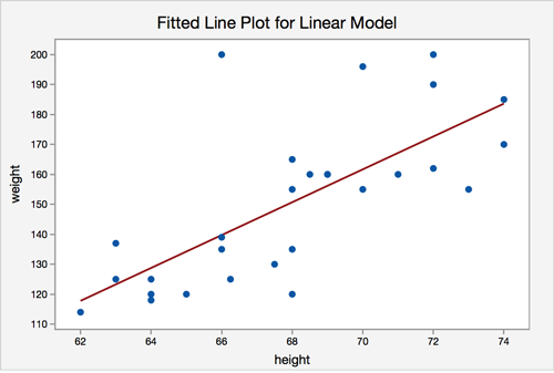
Fitted line plot for a linear model graph from Minitab. Height is on the x-axis and height is the y-axis. The data is scattered in a linear positive direction.

The scatterplot shows that, in general, as height increases, weight increases. There does not appear to be any clear violation that the relationship is not linear.

Assumption 2: Independence of errors - There is not a relationship between the residuals and weight.

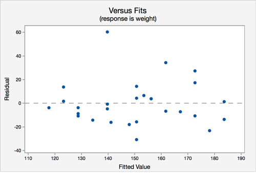
Versus fits graph from Minitab. Fitted value is on the x-axis and the residual is the y-axis. The data points have no clear pattern.

In the residuals versus fits plot, the points seem randomly scattered, and it does not appear that there is a relationship.

Assumption 3: Normality of errors - The residuals must be approximately normally distributed.

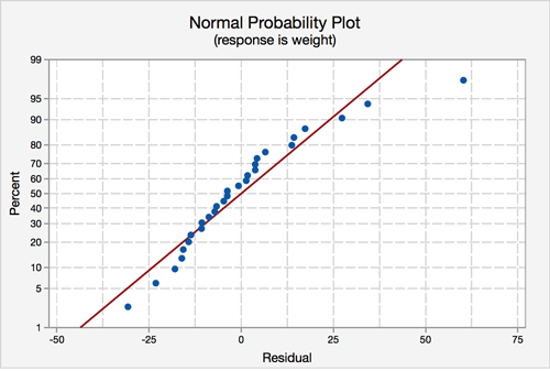
Normal probability plot from Minitab. The x-axis is the residual and the y-axis is the percent. The point are close to the line.

Most of the data points fall close to the line, but there does appear to be a slight curving. There is one data point that stands out.

Assumption 4: Equal Variances - The variance of the residuals is the same for all values of $X$.

Versus fits graph from Minitab. Fitted value is on the x-axis and the residual is the y-axis. The data points have no clear pattern.

In this plot, there does not seem to be a pattern.

All of the assumption except for the normal assumption seem valid.

9.2.4 - Inferences about the Population Slope

In this section, we will present the hypothesis test and the confidence interval for the population slope. A similar test for the population intercept, $\beta_0$, is not discussed in this class because it is not typically of interest.

Hypothesis Test for the Population Slope

Research Question	Is there a linear relationship?	Is there a positive linear relationship?	Is there a negative linear relationship?
Null Hypothesis	$\beta_1=0$	$\beta_1=0$	$\beta_1=0$
Alternative Hypothesis	$\beta_1\ne0$	$\beta_1>0$	$\beta_1<0$
Type of Test	Two-tailed, non-directional	Right-tailed, directional	Left-tailed, directional

The test statistic for the test of population slope is:

$t^*=\dfrac{\hat{\beta}_1}{\hat{SE}(\hat{\beta}_1)}$

where $\hat{SE}(\hat{\beta}_1)$ is the estimated standard error of the sample slope (found in Minitab output). Under the null hypothesis and with the assumptions shown in the previous section, $t^*$ follows a $t$-distribution with $n-2$ degrees of freedom.

Note! In this class, we will have Minitab perform the calculations for this test. Minitab's output gives the result for two-tailed tests for $\beta_1$ and $\beta_0$. If you wish to perform a one-sided test, you would have to adjust the p-value Minitab provides.

Confidence Interval for the Population Slope

$ (1-\alpha)100$% Confidence Interval for the Population Slope

The $ (1-\alpha)100$% confidence interval for $\beta_1$ is:

$\hat{\beta}_1\pm t_{\alpha/2}\left(\hat{SE}(\hat{\beta}_1)\right)$

where $t$ has $n-2$ degrees of freedom.

Note! The degrees of freedom of t depends on the number of independent variables. The degrees of freedom is $n - 2$ when there is only one independent variable.

9.2.5 - Other Inferences and Considerations

Inferences about Mean Response for New Observation

Let’s go back to the height and weight example:

Example

If you are asked to estimate the weight of a STAT 500 student, what will you use as a point estimate? If I tell you that the height of the student is 70 inches, can you give a better estimate of the person's weight?

Now that we have our regression equation, we can use height to provide a better estimate of weight. We would want to report a mean response value for the provided height, i.e 70 inches.

The mean response at a given X value is given by:

$E(Y)=\beta_0+\beta_1X$

This is an unknown but fixed value. The point estimate for mean response at $X=x$ is given by $\hat{\beta}_0+\hat{\beta}_1x$.

The example for finding this mean response for height and weight is shown later in the lesson.

Inferences about Outcome for New Observation

The point estimate for the outcome at $X = x$ is provided above. The interval to estimate the mean response is called the confidence interval. Minitab calculates this for us.

The interval used to estimate (or predict) an outcome is called prediction interval. For a given x value, the prediction interval and confidence interval have the same center, but the width of the prediction interval is wider than the width of the confidence interval. That makes good sense since it is harder to estimate a value for a single subject (say predict your weight based on your height) than it would be to estimate the average for subjects (say predict the mean weight of people who are your height). Again, Minitab will calculate this interval as well.

Cautions with Linear Regression

First, use extrapolation with caution. Extrapolation is applying a regression model to X-values outside the range of sample X-values to predict values of the response variable $Y$. For example, you would not want to use your age (in months) to predict your weight using a regression model that used the age of infants (in months) to predict their weight.

Second, the fact that there is no linear relationship (i.e. correlation is zero) does not imply there is no relationship altogether. The scatter plot will reveal whether other possible relationships may exist. The figure below gives an example where X, Y are related, but not linearly related i.e. the correlation is zero.

Outliers and Influential Observations

Influential observations are points whose removal causes the regression equation to change considerably. It is flagged by Minitab in the unusual observation list and denoted as X. Outliers are points that lie outside the overall pattern of the data. Potential outliers are flagged by Minitab in the unusual observation list and denoted as R.

The following is the Minitab output for the unusual observations within the height and weight example:

Fits and Diagnostics for Unusual Observations

Obs	weight	Fit	Residual	St Resid
24	200.00	139.74	60.26	3.23R

R Large Residual

Some observations may be both outliers and influential, and these are flagged by R and X (R X). Those observational points will merit particular attention. In our height and weight example, we have an R (potential outlier) observation, but it is not an influential point (RX observation).

Estimating the standard deviation of the error term

Our simple linear regression model is:

$Y=\beta_0+\beta_1X+\epsilon$

The errors for the $n$ observations are denoted as $\epsilon_i$, for $i=1, …, n$. One of our assumptions is that the errors have equal variance (or equal standard deviation). We can estimate the standard deviation of the error by finding the standard deviation of the residuals, $\epsilon_i=y_i-\hat{y}_i$. Minitab also provides the estimate for us, denoted as $S$, under the Model Summary. We can also calculate it by:

$s=\sqrt{\text{MSE}}$

Find the MSE in the ANOVA table, under the MS column and the Error row.

9.2.6 - Examples

In this section, we present an example and review what we have covered so far in the context of the example.

Example 9-5: Student height and weight (SLR)

We will continue with our height and weight example. Answer the following questions.

Is height a significant linear predictor of weight? Conduct the test at a significance level of 5%. State the regression equation.
Does $\beta_0$ have a meaningful interpretation?
Find the confidence interval for the population slope and interpret it in the context of the problem.
If a student is 70 inches, what weight could we expect?
What is the estimated standard deviation of the error?

Answer

The model for this problem is:
$\text{weight}=\beta_0+\beta_1\text{height}+\epsilon$
The hypotheses we are testing are:
$H_0\colon \beta_1=0$
$H_a\colon \beta_1\ne 0$
Recall that we previously examined the assumptions. Here is a summary of what we presented before:
Assumptions
1. Linearity: The relationship between height and weight must be linear.
  The scatterplot shows that, in general, as height increases, weight increases. There does not appear to be any clear violation that the relationship is not linear.
2. Independence of errors: There is not a relationship between the residuals and weight.
  In the residuals versus fits plot, the points seem randomly scattered, and it does not appear that there is a relationship.
3. Normality of errors: The residuals must be approximately normally distributed.
  Most of the data points fall close to the line, but there does appear to be a slight curving. There is one data point that clearly stands out. In the histogram, we can see that, with that one observation, the shape seems slightly right-skewed.
4. Equal variances: The variance of the residuals is the same for all values of $X$.
In this plot, there does not seem to be a pattern.
All of the assumption except for the normal assumption seem valid.
Minitab output for the height and weight data:
Model Summary
S
R-sq
R-sq(adj)
R-sq(pred)
19.1108
50.57%
48.67%
44.09%
Coefficients
Team
Coef
SE Coef
T-Value
P-Value
VIF
Constant
-222.5
72.4
-3.07
0.005

height
5.49
1.06
5.16
0.000
1.00
Regression Equation
$\hat{\text{weight}} = -222.5+5.49\text{height}$
The regression equation is:
$\hat{\text{weight}}=-222.5+5.49\text{height}$
The slope is 5.49, and the intercept is -222.5. The test for the slope has a p-value of less than 0.001. Therefore, with a significance level of 5%, we can conclude that there is enough evidence to suggest that height is a significant linear predictor of weight. We should make this conclusion with caution, however, since one of our assumptions might not be valid.
The intercept is -222.5. Therefore, when height is equal to 0, then a person’s weight is predicted to be -222.5 pounds. It is also not possible for someone to have a height of 0 inches. Therefore, the intercept does not have a valid meaning.
The confidence interval for the population slope is:
$\hat{\beta}_1\pm t_{\alpha/2}\hat{SE}(\hat{\beta}_1)$
The estimate for the slope is 5.49 and the standard error for the estimate (SE Coef in the output) is 1.06. There are $n=28$ observations so the degrees of freedom are $28-2=26$. Using Minitab, we find the t-value to be 2.056. Putting the pieces together, the interval is:
$5.49\pm 2.056(1.06)$
$(3.31, 7.67)$
We are 95% confident that the population slope is between 3.31 and 7.67. In other words, we are 95% confident that, as height increases by one inch, that weight increases by between 3.31 and 7.67 pounds, on average.
Using the regression formula with a height equal to 70 inches, we get:
$\hat{\text{weight}}=-222.5+5.49(70)=161.8$
A student with a height of 70 inches, we would expect a weight of 162.3 pounds. If we wanted, we could have Minitab produce a confidence interval for this estimate. We will leave this out for this example.
Using the output, under the model summary:
$s=19.1108$

S	R-sq	R-sq(adj)	R-sq(pred)
19.1108	50.57%	48.67%	44.09%

Team	Coef	SE Coef	T-Value	P-Value	VIF
Constant	-222.5	72.4	-3.07	0.005
height	5.49	1.06	5.16	0.000	1.00

Try it!

The No-Lemon used car dealership in a college town records the age (in years) and price for cars it sold in the last year (cars_sold.txt). Here is a table of this data.

age	4	4	4	5	5	6	7	7	8
price	6200	5700	6800	5600	4500	4900	4600	4300	4200

age	8	8	9	9	10	10	11	12	13
price	4500	4000	3200	3100	2500	2100	2600	2400	2200

Using the data above, answer the following questions.

Is age a significant negative linear predictor of price? Conduct the test at a significance level of 5%.
Does $\beta_0$ have a meaningful interpretation?
Find the confidence interval for the population slope and interpret it in context of the problem.
If a car is seven years old, what price could we expect?
What is the estimate of the standard deviation of the errors?

The linear regression model is:

$\text{price}=\beta_0+\beta_1\text{age}+\epsilon$

To test whether age is a statistically significant negative linear predictor of price, we can set up the following hypotheses:.

$H_0\colon \beta_1=0$

$H_a\colon \beta_1< 0$

We need to verify that our assumptions are satisfied. Let's do this in Minitab. Remember, we have to run the linear regression analysis to check the assumptions.

Assumption 1: Linearity

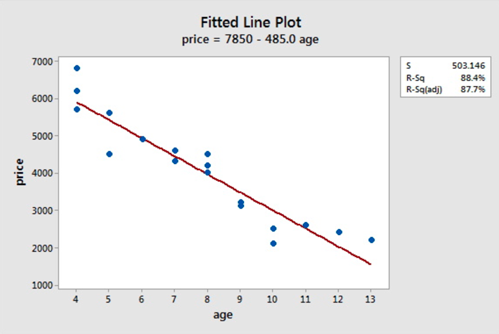
Fitted line plot that shows the scatter plot of a car's age versus it's price. The graph is linear with a negative slope.

The scatterplot below shows that the relationship between age and price scores is linear. There appears to be a strong negative linear relationship and no obvious outliers.

Assumption 2: Independence of errors

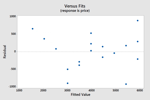
Versus fits graph from Minitab. Fitted value is on the x-axis and the residual is the y-axis.

There does not appear to be a relationship between the residuals and the fitted values. Thus, this assumption seems valid.

Assumption 3: Normality of errors

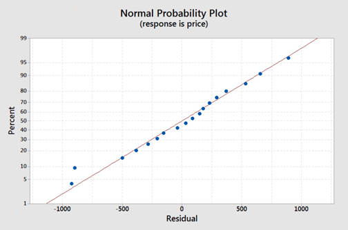
Versus order graph from Minitab. The observation order is the x-axis and the residual is the y-axis.

On the normal probability plot we are looking to see if our observations follow the given line. This graph does not indicate that there is a violation of the assumption that the errors are normal. If a probability plot is not an option we can refer back to one of our first lessons on graphing quantitative data and use a histogram or boxplot to examine if the residuals appear to follow a bell shape.

Assumption 4: Equal Variances

Normal probability plot from Minitab. The x-axis is the residual and the y-axis is the percent. The point are close to the line.

Again we will use the plot of residuals versus fits. Now we are checking that the variance of the residuals is consistent across all fitted values. This assumption seems valid.

Model Summary

S	R-sq	R-sq(adj)	R-sq(pred)
503.146	88.39%	87.67%	84.41%

Coefficients

Team	Coef	SE Coef	T-Value	P-Value	VIF
Constant	7850	362	21.70	0.000
age	-485.0	43.9	-11.04	0.000	1.00

Regression Equation

$\hat{\text{price}} = 7850 - 485.0 \text{age}$

From the output above we can see that the p-value of the coefficient of age is 0.000 which is less than 0.001. The Minitab output is for a two-tailed test and we are dealing with a left-tailed test. Therefore, the p-value for the left-tailed test is less than $\frac{0.001}{2}$ or less than 0.0005.

We can thus conclude that age (in years) is a statistically significant negative linear predictor of price for any reasonable $\alpha$ value.

$\beta_0$ is the y-intercept, which means it is the value of price when age is equal to 0. It is possible for a vehicle to have number of years equal to 0. Therefore, it does have an interpretable meaning. We should use caution if we use this model to predict the price of a car with age equal to 0 because it is outside the range of values used to estimate the model.

The 95% confidence interval for the population slope is:

$\hat{\beta}_1\pm t_{\alpha/2}\text{SE}(\hat{\beta}_1)$

Using the output, $\hat{\beta}_1=-485$ and the $\text{SE}(\hat{\beta}_1)=43.9$. We need to have $t_{\alpha/2}$ with $n-2$ degrees of freedom. In this case, there are 18 observations so the degrees of freedom are $18-2=16$. Using software, we find $t_{\alpha/2}=2.12$.

The 95% confidence interval is:

$-485\pm 2.12(43.9)$

$(-578.068, -391.932)$

We are 95% confident that the population slope for the regression model is between -578.068 and -391.932. In other words, we are 95% confident that, for every one year increase in age, the price of a vehicle will decrease between 391.932 and 578.068 dollars.

We can use the regression equation with $\text{age}=7$:

$\hat{\text{price}}=7850-485(7)=4455$

We can expect the price to be $4455.

The residual standard error is estimated by s, which is calculated as:

$s=\sqrt{\text{MSE}}=\sqrt{253156}=503.146$

Note! The MSE is found in the ANOVA table that is part of the regression output in Minitab.

It is also shown as $s$ under the model summary in the output.

^[1]	Link
↥	Has Tooltip/Popover
	Toggleable Visibility

Research Question	Is there a linear relationship?	Is there a positive linear relationship?	Is there a negative linear relationship?
Null Hypothesis	\(\beta_1=0\)	\(\beta_1=0\)	\(\beta_1=0\)
Alternative Hypothesis	\(\beta_1\ne0\)	\(\beta_1>0\)	\(\beta_1<0\)
Type of Test	Two-tailed, non-directional	Right-tailed, directional	Left-tailed, directional

9.2 - Simple Linear Regression

9.2.1 - The SLR Model

\(\hat{\beta}_0\) (The constant term)

9.2.2 - Interpreting the Coefficients

Example 9-3: Student height and weight (Interpreting the coefficients)

9.2.3 - Assumptions for the SLR Model

Assumptions for Simple Linear Regression

Example 9-4: Student height and weight (SLR Assumptions)

9.2.4 - Inferences about the Population Slope

9.2.5 - Other Inferences and Considerations

Inferences about Mean Response for New Observation

Example

Inferences about Outcome for New Observation

Cautions with Linear Regression

Outliers and Influential Observations

Estimating the standard deviation of the error term

9.2.6 - Examples

Example 9-5: Student height and weight (SLR)

Model Summary

Coefficients

Regression Equation

Try it!

Model Summary

Coefficients

Regression Equation