10.2 - A Statistical Test for One-Way ANOVA

Hypotheses

Before we go into the details of the test, we need to determine the null and alternative hypotheses. Recall that for a test for two independent means, the null hypothesis was \(\mu_1=\mu_2\). In one-way ANOVA, we want to compare \(t\) population means, where \(t>2\). Therefore, the null hypothesis for analysis of variance for \(t\) population means is:

\(H_0\colon \mu_1=\mu_2=...\mu_t\)

The alternative, however, cannot be set up similarly to the two-sample case. If we wanted to see if two population means are different, the alternative would be \(\mu_1\ne\mu_2\). With more than two groups, the research question is “Are some of the means different?." If we set up the alternative to be \(\mu_1\ne\mu_2\ne…\ne\mu_t\), then we would have a test to see if ALL the means are different. This is not what we want. We need to be careful how we set up the alternative. The mathematical version of the alternative is...

\(H_a\colon \mu_i\ne\mu_j\text{ for some }i \text{ and }j \text{ where }i\ne j\)

This means that at least one of the pairs is not equal. The more common presentation of the alternative is:

\(H_a\colon \text{ at least one mean is different}\) or \(H_a\colon \text{ not all the means are equal}\)

Test Statistic

Recall that when we compare the means of two populations for independent samples, we use a 2-sample t-test with pooled variance when the population variances can be assumed equal.

Test Statistic for One-Way ANOVA

For more than two populations, the test statistic, \(F\), is the ratio of between group sample variance and the within-group-sample variance. That is,

\(F=\dfrac{\text{between group variance}}{\text{within group variance}}\)

Under the null hypothesis (and with certain assumptions), both quantities estimate the variance of the random error, and thus the ratio should be close to 1. If the ratio is large, then we have evidence against the null, and hence, we would reject the null hypothesis.

In the next section, we present the assumptions for this test. In the following section, we present how to find the between group variance, the within group variance, and the F-statistic in the ANOVA table.

10.2.1 - ANOVA Assumptions

Assumptions for One-Way ANOVA Test

There are three primary assumptions in ANOVA:

The responses for each factor level have a normal population distribution.
These distributions have the same variance.
The data are independent.

Note! Violations to the first two that are not extreme can be considered not serious. The sampling distribution of the test statistic is fairly robust, especially as sample size increases and more so if the sample sizes for all factor levels are equal. If you conduct an ANOVA test, you should always try to keep the same sample sizes for each factor level.

A general rule of thumb for equal variances is to compare the smallest and largest sample standard deviations. This is much like the rule of thumb for equal variances for the test for independent means. If the ratio of these two sample standard deviations falls within 0.5 to 2, then it may be that the assumption is not violated.

Example 10-1: Tar Content Comparisons

Recall the application from the beginning of the lesson. We wanted to see whether the tar contents (in milligrams) for three different brands of cigarettes were different. Lab Precise and Lab Sloppy each took six samples from each of the three brands (A, B and C). Check the assumptions for this example.

Answer

Lab Precise

The sample size is small. We should check for obvious violations using the Normal Probability Plot.
The graph shows no obvious violations from Normal, but we should proceed with caution.

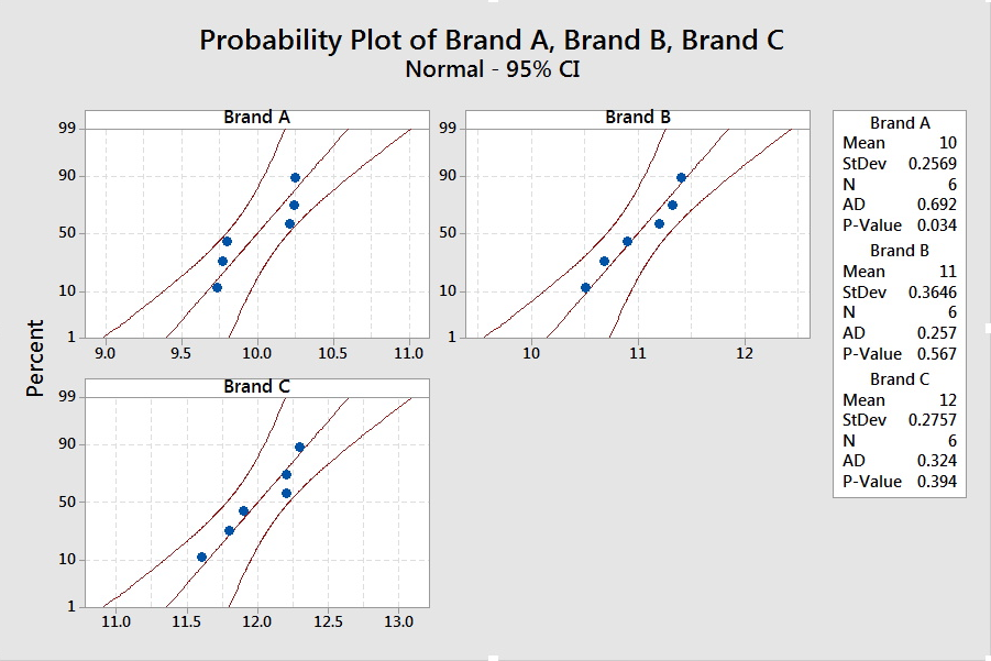
The summary statistics for the three brands are presented.

Descriptive Statistics: Precise Brand A, Precise Brand B, Precise Brand C

Variable	Mean	StDev
Precise Brand A	10.000	0.257
Precise Brand B	11.000	0.365
Precise Brand C	12.000	0.276

The smallest standard deviation is 0.257, and twice the value is 0.514. The largest standard deviation is less than this value. Since the sample sizes are the same, it is safe to assume the standard deviations (and thus the variances) are equal.

The samples were taken independently, so there is no indication that this assumption is violated.

Lab Sloppy

The sample size is small. We should check for obvious violations using the Normal Probability Plot.

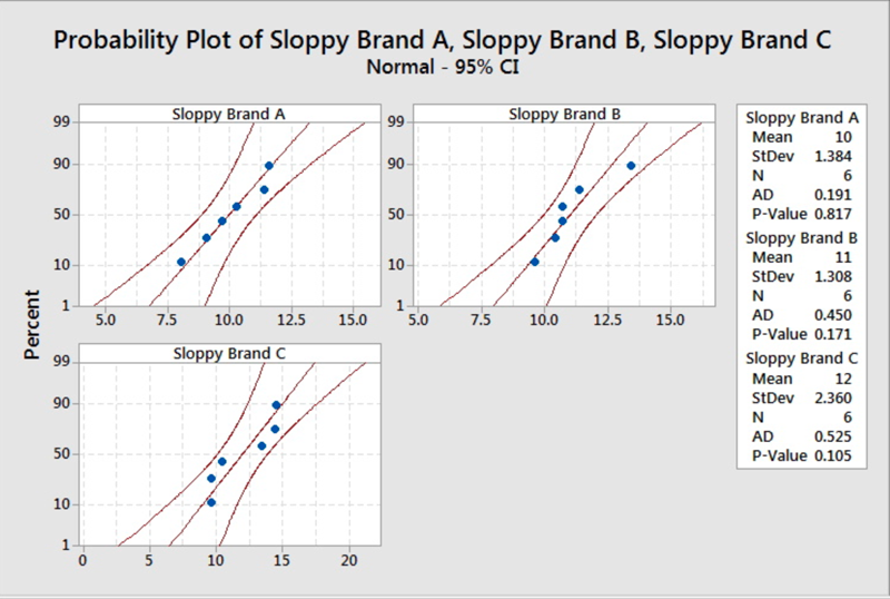
The summary statistics for the three brands are presented.

Descriptive Statistics: Sloppy Brand A, Sloppy Brand B, Sloppy Brand C

Variable	Mean	StDev
Sloppy Brand A	10.000	1.384
Sloppy Brand B	11.000	1.308
Sloppy Brand C	12.000	2.360

The smallest standard deviation is 1.308, and twice the value is 2.616. The largest standard deviation is less than this value. Since the sample sizes are the same, it is safe to assume the standard deviations (and thus the variances) are equal.

The samples were taken independently, so there is no indication that this assumption is violated.

10.2.2 - The ANOVA Table

In this section, we present the Analysis of Variance Table for a completely randomized design, such as the tar content example.

Data Table

Random samples of size \(n_1, …, n_t\) are drawn from the respective \(t\) populations. The data would have the following format:

Population	Data				Mean
1	\(y_{11}\)	\(y_{12}\)	...	\(y_{1n_1}\)	\(\bar{y}_{1.}\)
2	\(y_{21}\)	\(y_{22}\)	...	\(y_{2n_2}\)	\(\bar{y}_{2.}\)
⋮	⋮	⋮	⋮	⋮	⋮
\(t\)	\(y_{t1}\)	\(y_{t2}\)	...	\(y_{tn_t}\)	\(\bar{y}_{t.}\)

Notation

\(t\): The total number of groups

\(y_{ij}\): The \(j^{th}\) observation from the \(i^{th}\) population.

\(n_i\): The sample size from the \(i^{th}\) population.

\(n_T\): The total sample size: \(n_T=\sum_{i=1}^t n_i\).

\(\bar{y}_{i.}\): The mean of the sample from the \(i^{th}\) population.

\(\bar{y}_{..}\): The mean of the combined data. Also called the overall mean.

Recall that we want to examine the between group variation and the within group variation. We can find an estimate of the variations with the following:

Sum of Squares for Treatment or the Between Group Sum of Squares: \(\text{SST}=\sum_{i=1}^t n_i(\bar{y}_{i.}-\bar{y}_{..})^2\)
Sum of Squares for Error or the Within Group Sum of Squares: \(\text{SSE}=\sum_{i, j} (y_{ij}-\bar{y}_{i.})^2\)
Total Sum of Squares: \(\text{TSS}=\sum_{i,j} (y_{ij}-\bar{y}_{..})^2\)

It can be derived that \(\text{TSS } = \text{ SST } + \text{ SSE}\).

We can set up the ANOVA table to help us find the F-statistic. Hover over the light bulb to get more information on that item.

The ANOVA Table

Source	Df	SS	MS	F
Treatment	\(t-1\)	\(\text{SST}\)	\(\text{MST}=\dfrac{\text{SST}}{t-1}\)	\(\dfrac{\text{MST}}{\text{MSE}}\)
Error	\(n_T-t\)	\(\text{SSE}\)	\(\text{MSE}=\dfrac{\text{SSE}}{n_T-t}\)
Total	\(n_T-1\)	\(\text{TSS}\)

The p-value is found using the F-statistic and the F-distribution. We will not ask you to find the p-value for this test. You will only need to know how to interpret it. If the p-value is less than our predetermined significance level, we will reject the null hypothesis that all the means are equal.

The ANOVA table can easily be obtained by statistical software and hand computation of such quantities are very tedious.

^[1]	Link
↥	Has Tooltip/Popover
	Toggleable Visibility