12 Multicollinearity & Other Regression Pitfalls

Multicollinearity

Uncorrelated predictors

Highly correlated predictors

Overview

So far, in our study of multiple regression models, we have ignored something that we probably shouldn’t have — and that’s what is called multicollinearity. We’re going to correct our blissful ignorance in this lesson.

Multicollinearity exists when two or more of the predictors in a regression model are moderately or highly correlated. Unfortunately, when it exists, it can wreak havoc on our analysis and thereby limit the research conclusions we can draw. As we will soon learn, when multicollinearity exists, any of the following pitfalls can be exacerbated:

the estimated regression coefficient of any one variable depends on which other predictors are included in the model
the precision of the estimated regression coefficients decreases as more predictors are added to the model
the marginal contribution of any one predictor variable in reducing the error sum of squares depends on which other predictors are already in the model
hypothesis tests for $\beta_k = 0$ may yield different conclusions depending on which predictors are in the model

In this lesson, we’ll take a look at an example or two that illustrates each of the above outcomes. Then, we’ll spend some time learning how not only to detect multicollinearity but also how to reduce it once we’ve found it.

We’ll also consider other regression pitfalls, including extrapolation, nonconstant variance, autocorrelation, overfitting, excluding important predictor variables, missing data, power, and sample size.

Objectives

Upon completion of this lesson, you should be able to:

Distinguish between structural multicollinearity and data-based multicollinearity.
Know what multicollinearity means.
Understand the effects of multicollinearity on various aspects of regression analyses.
Understand the effects of uncorrelated predictors on various aspects of regression analyses.
Understand variance inflation factors, and how to use them to help detect multicollinearity.
Know the two ways of reducing data-based multicollinearity.
Understand how centering the predictors in a polynomial regression model helps to reduce structural multicollinearity.
Know the main issues surrounding other regression pitfalls, including extrapolation, nonconstant variance, autocorrelation, overfitting, excluding important predictor variables, missing data, and power, and sample size.

12.1 What is Multicollinearity?

As stated in the lesson overview, multicollinearity exists whenever two or more of the predictors in a regression model are moderately or highly correlated. Now, you might be wondering why can’t a researcher just collect his data in such a way to ensure that the predictors aren’t highly correlated. Then, multicollinearity wouldn’t be a problem, and we wouldn’t have to bother with this silly lesson.

Unfortunately, researchers often can’t control the predictors. Obvious examples include a person’s gender, race, grade point average, math SAT score, IQ, and starting salary. For each of these predictor examples, the researcher just observes the values as they occur for the people in her random sample.

Multicollinearity happens more often than not in such observational studies. And, unfortunately, regression analyses most often take place on data obtained from observational studies. If you aren’t convinced, consider the example data sets for this course. Most of the data sets were obtained from observational studies, not experiments. It is for this reason that we need to fully understand the impact of multicollinearity on our regression analyses.

Types of multicollinearity

Structural multicollinearity is a mathematical artifact caused by creating new predictors from other predictors — such as creating the predictor $x^{2}$ from the predictor $x$.
Data-based multicollinearity, on the other hand, is a result of a poorly designed experiment, reliance on purely observational data, or the inability to manipulate the system on which the data are collected.

In the case of structural multicollinearity, the multicollinearity is induced by what you have done. Data-based multicollinearity is the more troublesome of the two types of multicollinearity. Unfortunately, it is the type we encounter most often!

Example 12.1 (Blood Pressure Data) Let’s take a quick look at an example in which data-based multicollinearity exists. Some researchers observed — notice the choice of word! — the following Blood Pressure data on 20 individuals with high blood pressure:

blood pressure ($y = BP$, in mm Hg)
age ($x_{1} = Age,$ in years)
weight ($x_{2} = Weight,$ in kg)
body surface area ($x_{3} = BSA,$ in sq m)
duration of hypertension ($x_{4} = Dur,$ in years)
basal pulse ($x_{5} = Pulse,$ in beats per minute)
stress index ($x_{6} = Stress$)

The researchers were interested in determining if a relationship exists between blood pressure and age, weight, body surface area, duration, pulse rate, and/or stress level.

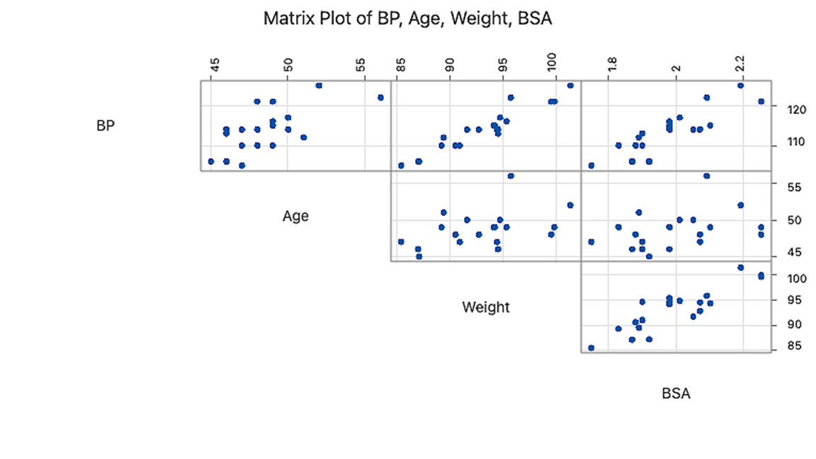
The matrix plot of BP, Age, Weight, and BSA:

and the matrix plot of BP, Dur, Pulse, and Stress:

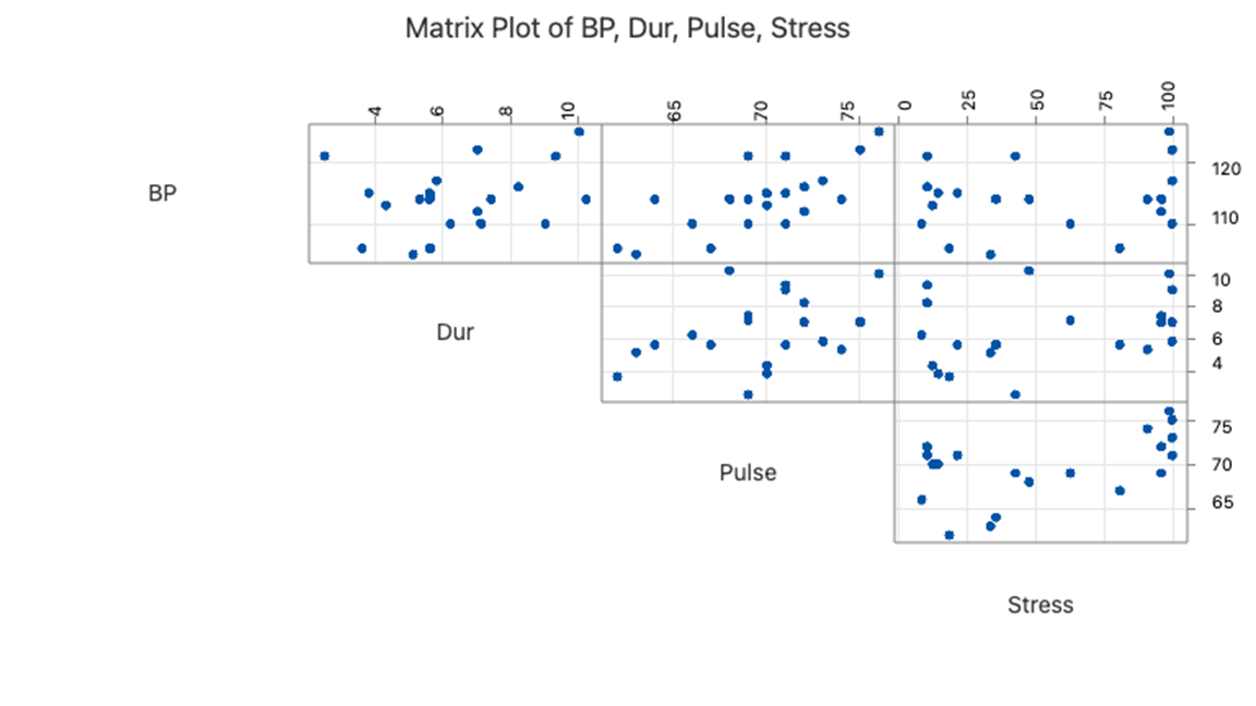
allow us to investigate the various marginal relationships between the response BP and the predictors. Blood pressure appears to be related fairly strongly to Weight and BSA, and hardly related at all to the Stress level.

The matrix plots also allow us to investigate whether or not relationships exist among the predictors. For example, Weight and BSA appear to be strongly related, while Stress and BSA appear to be hardly related at all.

The following correlation matrix:

Correlation: BP, Age, Weight, BSA, Dur, Pulse, Stress

BP		Age	Weight	BSA	Dur	Pulse
Age	0.659
Weight	0.950	0.407
BSA	0.866	0.378	0.875
Dur	0.293	0.344	0.201	0.131
Pulse	0.721	0.619	0.659	0.465	0.402
Stress	0.164	0.368	0.034	0.018	0.312	0.506

provides further evidence of the above claims. Blood pressure appears to be related fairly strongly to Weight ($r$ = 0.950) and BSA ($r$ = 0.866), and hardly related at all to Stress level ($r$ = 0.164). And, Weight and BSA appear to be strongly related ($r$ = 0.875), while Stress and BSA appear to be hardly related at all ($r$ = 0.018). The high correlation among some of the predictors suggests that data-based multicollinearity exists.

Now, what we need to learn is the impact of multicollinearity on regression analysis. Let’s go do it!

12.2 Uncorrelated Predictors

In order to get a handle on this multicollinearity thing, let’s first investigate the effects that uncorrelated predictors have on regression analyses. To do so, we’ll investigate a “contrived” data set, in which the predictors are perfectly uncorrelated. Then, we’ll investigate the second example of a “real” data set, in which the predictors are nearly uncorrelated. Our two investigations will allow us to summarize the effects that uncorrelated predictors have on regression analyses.

Then, on the next page, we’ll investigate the effects that highly correlated predictors have on regression analyses. In doing so, we’ll learn — and therefore be able to summarize — the various effects multicollinearity has on regression analyses.

What is the effect on regression analyses if the predictors are perfectly uncorrelated?

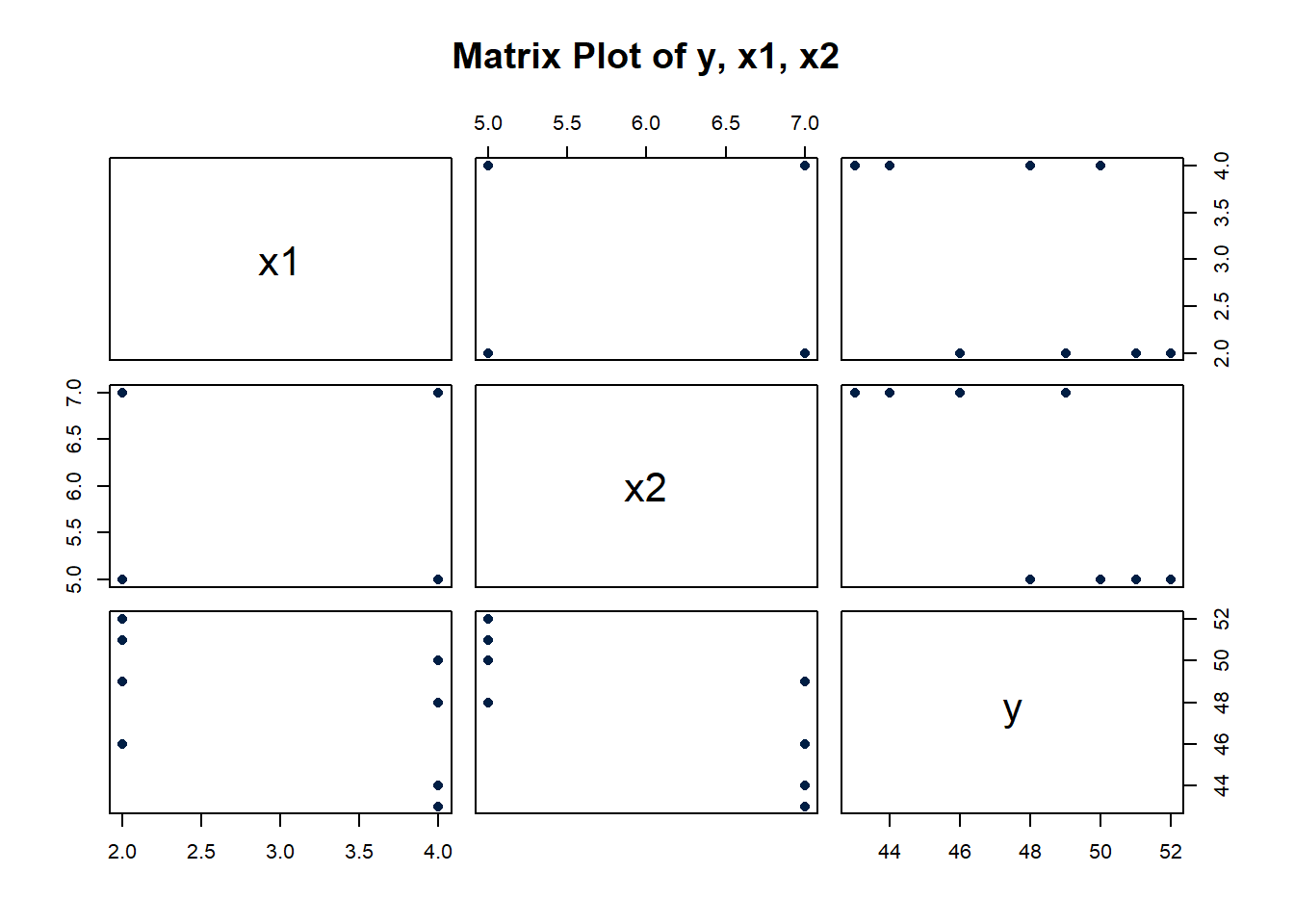
Consider the following matrix plot of the response $y$ and two predictors $x_{1}$ and $x_{2},$ of a contrived data set (Uncorrelated Predictors data set), in which the predictors are perfectly uncorrelated:

Scatterplot matrix plot of y, x1, and x2 — Fig 12.3: Matrix Plot of y, x1, x2

As you can see there is no apparent relationship at all between the predictors $x_{1}$ and $x_{2}.$ That is, the correlation between $x_{1}$ and $x_{2}$ is zero:

Pearson correlation of x1 and x2 = 0.000

suggesting the two predictors are perfectly uncorrelated.

Now, let’s just proceed quickly through the output of a series of regression analyses collecting various pieces of information along the way. When we’re done, we’ll review what we learned by collating the various items in a summary table.

The regression of the response $y$ on the predictor $x_{1}$:

Regression Analysis: y versus x1

Analysis of Variance

Source	DF	Seq SS	Seq MS	F-Value	P-Value
Regression	1	21.13	21.125	2.36	0.176
x1	1	21.13	21.125	2.36	0.176
Error	6	53.75	8.958
Total	7	74.88

Model Summary

S	R-sq	R-sq(adj)	R-sq(pred)
2.99305	28.21%	16.25%	0.00%

Coefficients

Term	Coef	SE Coef	T-Value	P-Value	VIF
Constant	52.75	3.35	15.76	0.000
x1	-1.62	1.06	-1.54	0.176	1.00

Regression Equation

y = 52.75 - 1.62 x1

yields the estimated coefficient $b_{1}$ = -1.62, the standard error $se(b_{1})$ = 1.06, and the regression sum of squares $SSR(x_{1})$ = 21.13.

The regression of the response $y$ on the predictor $x_{2}$:

Regression Analysis: y versus x2

Analysis of Variance

Source	DF	Seq SS	Seq MS	F-Value	P-Value
Regression	1	45.13	45.125	9.10	0.023
x2	1	45.13	45.125	9.10	0.023
Error	6	29.75	4.958
Total	7	74.88

Model Summary

S	R-sq	R-sq(adj)	R-sq(pred)
2.22673	60.27%	53.64%	29.36%

Coefficients

Term	Coef	SE Coef	T-Value	P-Value	VIF
Constant	62.13	4.79	12.97	0.000
x2	-2.375	0.787	-3.02	0.023	1.00

Regression Equation

y = 62.13 - 2.375 x2

yields the estimated coefficient $b_{2}$ = -2.375, the standard error $se(b_{2})$ = 0.787, and the regression sum of squares $SSR(x_{2})$ = 45.13.

The regression of the response $y$ on the predictors $x_{1}$ and $x_{2}$ (in that order):

Regression Analysis: y versus x1, x2

Analysis of Variance

Source	DF	Seq SS	Seq MS	F-Value	P-Value
Regression	2	66.250	33.125	19.20	0.005
x1	1	21.125	21.125	12.25	0.017
x2	1	45.125	45.125	26.16	0.004
Error	5	8.625	1.725
Lack-of-Fit	1	1.125	1.125	0.60	0.482
Pure Error	4	7.500	1.875
Total	7	74.875

Model Summary

S	R-sq	R-sq(adj)	R-sq(pred)
1.31339	88.48%	83.87%	70.51%

Coefficients

Term	Coef	SE Coef	T-Value	P-Value	VIF
Constant	67.00	3.15	21.27	0.000
x1	-1.625	0.464	-3.50	0.017	1.00
x2	-2.375	0.464	-5.11	0.004	1.00

Regression Equation

y = 67.00 - 1.625 x1 - 2.375 x2

yields the estimated coefficients $b_{1}$ = -1.625 and $b_{2}$ = -2.375, the standard errors se($b_{1}$) = 0.464 and se($b_{2}$) = 0.464, and the sequential sum of squares SSR($x_{2}$|$x_{1}$) = 45.125.

The regression of the response $y$ on the predictors $x_{2 }$ and $x_{1}$ (in that order):

Regression Analysis: y versus x2, x1

Analysis of Variance

Source	DF	Seq SS	Seq MS	F-Value	P-Value
Regression	2	66.250	33.125	19.20	0.005
x2	1	45.125	45.125	26.16	0.004
x1	1	21.125	21.125	12.25	0.017
Error	5	8.625	1.725
Lack-of-Fit	1	1.125	1.125	0.60	0.482
Pure Error	4	7.500	1.875
Total	7	74.875

Model Summary

S	R-sq	R-sq(adj)	R-sq(pred)
1.31339	88.48%	83.87%	70.51%

Coefficients

Term	Coef	SE Coef	T-Value	P-Value	VIF
Constant	67.00	3.15	21.27	0.000
x2	-2.375	0.464	-5.11	0.004	1.00
x1	-1.625	0.464	-3.50	0.017	1.00

Regression Equation

y = 67.00 - 2.375 x2 - 1.625 x1

yields the estimated coefficients $b_{1}$ = -1.625 and $b_{2}$ = -2.375, the standard errors $se(b_{1})$ = 0.464 and $se(b_{2})$ = 0.464, and the sequential sum of squares $SSR(x_{1}|x_{2})$ = 21.125.

Okay — as promised — compiling the results in a summary table, we obtain:

Model	$b_1$	$se(b_1)$	$b_2$	$se(b_2)$	Seq SS
$x_1$ only	-1.62	1.06	—	—	$SSR(x_1)$ 21.125
$x_2$ only	—	—	-2.375	0.787	$SSR(x_2)$ 45.125
$x_1, x_2$ (in order)	-1.625	0.464	-2.375	0.464	$SSR(x_2\|x_1)$ 41.125
$x_2, x_1$ (in order)	-1.625	0.464	-2.375	0.464	$SSR(x_1\|x_2)$ 21.125

What do we observe?

The estimated slope coefficients $b_{1}$ and $b_{2}$ are the same regardless of the model used.
The standard errors $se(b_{1})$ and $se(b_{2})$ don’t change much at all from model to model.
The sum of squares $SSR(x_{1})$ is the same as the sequential sum of squares $SSR(x_{1}|x_{2})$. The sum of squares $SSR(x_{2})$ is the same as the sequential sum of squares $SSR(x_{2}|x_{1})$.

These all seem to be good things! Because the slope estimates stay the same, the effect on the response ascribed to a predictor doesn’t depend on the other predictors in the model. Because $SSR(x_{1}) = SSR(x_{1}|x_{2})$, the marginal contribution that $x_{1}$ has in reducing the variability in the response $y$ doesn’t depend on the predictor $x_{2}.$ Similarly, because $SSR(x_{2}) = SSR(x_{2}|x_{1})$, the marginal contribution that $x_{2}$ has in reducing the variability in the response $y$ doesn’t depend on the predictor $x_{1}.$

These are the things we can hope for in regression analysis — but, then reality sets in! Recall that we obtained the above results for a contrived data set, in which the predictors are perfectly uncorrelated. Do we get similar results for real data with only nearly uncorrelated predictors? Let’s see!

What is the effect on regression analyses if the predictors are nearly uncorrelated?

To investigate this question, let’s go back and take a look at the blood pressure data set Blood Pressure data set. In particular, let’s focus on the relationships among the response $y = BP$ and the predictors $x_{3}$ = BSA and $x_{6}$ = Stress:

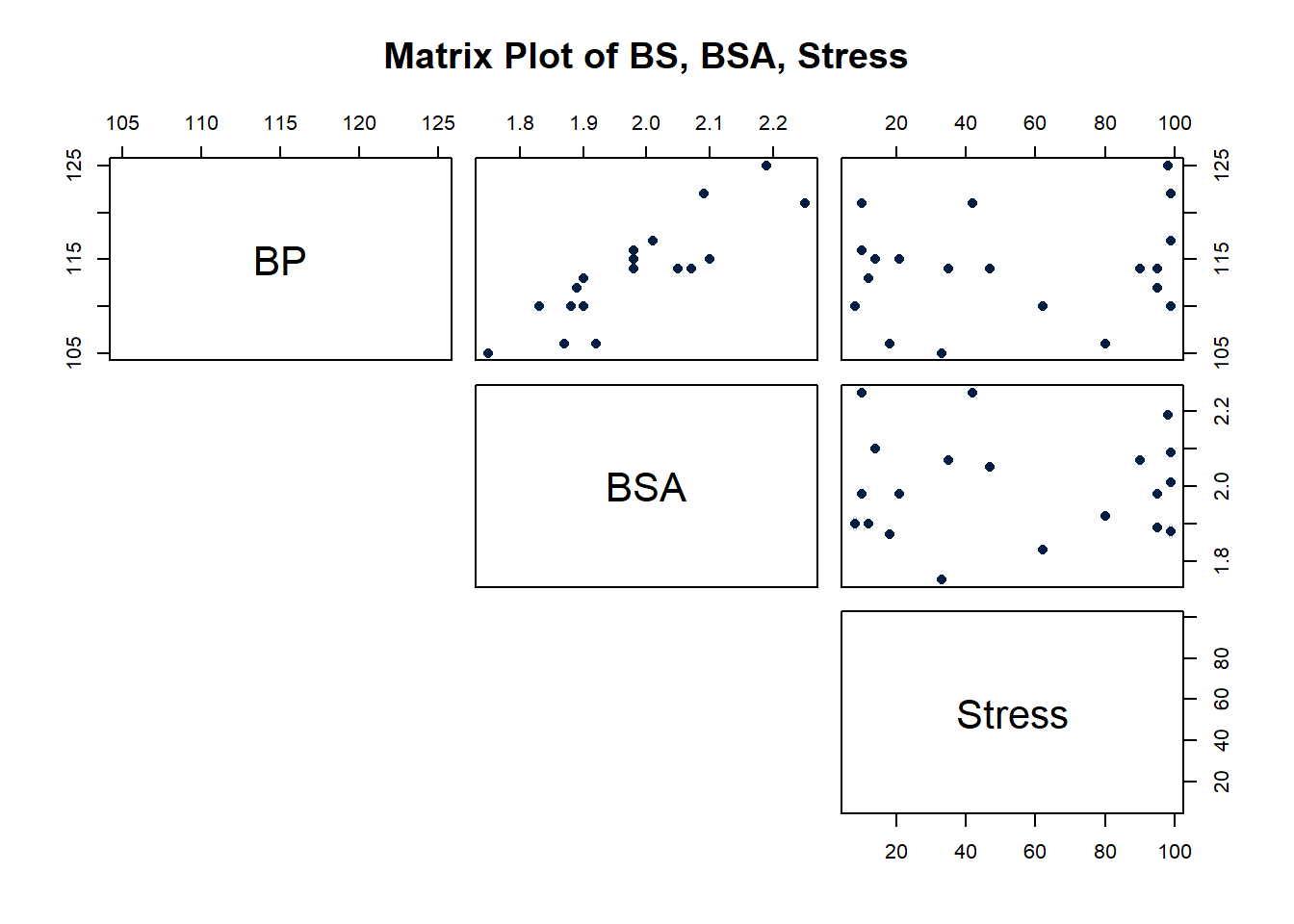
Scatterplot matrix plot of BP, BSA, Stress — Fig 12.4: Matrix Plot of BP, BSA, Stress

As the above matrix plot and the following correlation matrix suggest:

Correlation: BP, Age, Weight, BSA, Dur, Pulse, Stress

	BP	Age	Weight	BSA	Dur	Pulse
Age	0.659
Weight	0.950	0.407
BSA	0.866	0.378	0.875
Dur	0.293	0.344	0.201	0.131
Pulse	0.721	0.619	0.659	0.465	0.402
Stress	0.164	0.368	0.034	0.018	0.312	0.506

there appears to be a strong relationship between $y = BP$ and the predictor $x_{3}$ = BSA ($r$ = 0.866), a weak relationship between $y = BP$ and $x_{6}$ = Stress ($r$ = 0.164), and an almost non-existent relationship between $x_{3}$ = BSA and $x_{6}$ = Stress ($r$ = 0.018). That is, the two predictors are nearly perfectly uncorrelated.

What effect do these nearly perfectly uncorrelated predictors have on regression analyses? Let’s proceed similarly through the output of a series of regression analyses collecting various pieces of information along the way. When we’re done, we’ll review what we learned by collating the various items in a summary table.

The regression of the response $y = BP$ on the predictor $x_{6} = Stress$:

Analysis of Variance

Source	DF	Seq SS	Seq MS	F-Value	P-Value
Regression	1	15.04	15.04	0.50	0.490
Stress	1	15.04	15.04	0.50	0.490
Error	18	544.96	30.28
Lack-of-Fit	14	457.79	32.70	1.50	0.374
Pure Error	4	87.17	21.79
Total	19	560.00

Coefficients

Term	Coef	SE Coef	T-Value	P-Value	VIF
Constant	112.72	2.19	51.39	0.000
Stress	0.0240	0.0340	0.70	0.490	1.00

Regression Equation

BP = 112.72 + 0.0240 Stress

yields the estimated coefficient $b_{6}$ = 0.0240, the standard error $se(b_{6})$ = 0.0340, and the regression sum of squares $SSR(x_{6})$ = 15.04.

The regression of the response $y = BP$ on the predictor $x_{3}= BSA$:

Analysis of Variance

Source	DF	Seq SS	Seq MS	F-Value	P-Value
Regression	1	419.858	419.858	53.93	0.000
BSA	1	419.858	419.858	53.93	0.000
Error	18	140.142	7.786
Lack-of-Fit	13	133.642	10.280	7.91	0.016
Pure Error	5	6.500	1.300
Total	19	560.000

Coefficients

Term	Coef	SE Coef	T-Value	P-Value	VIF
Constant	49.50	4.65	10.63	0.000

BSA	34.44	4.69	7.34	0.000	1.00

Regression Equation

BP = 45.18 + 34.44 BSA

yields the estimated coefficient $b_{3}$ = 34.44, the standard error $se(b_{3}) = 4.69$, and the regression sum of squares $SSR(x_{3})$ = 419.858.

The regression of the response $y = BP$ on the predictors $x_{6} = Stress$ and $x_{3} = BSA$ (in that order):

Analysis of Variance

Source	DF	Seq SS	Seq MS	F-Value	P-Value
Regression	2	432.12	216.058	28.72	0.000
Stress	1	15.04	15.044	2.00	0.175
BSA	1	417.07	417.073	55.44	0.000
Error	17	127.88	7.523
Total	19	560.00

Coefficients

Term	Coef	SE Coef	T-Value	P-Value	VIF
Constant	44.24	9.26	4.78	0.000
Stress	0.0217	0.0170	1.28	0.219	1.00
BSA	34.33	4.61	7.45	0.000	1.00

Regression Equation

y = 44.24 + 0.0217 Stress + 34.33 BSA

yields the estimated coefficients $b_{6}$ = 0.0217 and $b_{3}$ = 34.33, the standard errors $se(b_{6})$ = 0.0170 and $se(b_{2})$ = 4.61, and the sequential sum of squares $SSR(x_{3}|x_{6})$ = 417.07.

Finally, the regression of the response $y = BP$ on the predictors $x_{3 } = BSA$ and $x_{6} = Stress$ (in that order):

Analysis of Variance

Source	DF	Seq SS	Seq MS	F-Value	P-Value
Regression	2	432.12	216.058	28.72	0.000
BSA	1	419.86	419.858	55.81	0.000
Stress	1	12.26	12.259	1.63	0.219
Error	6	104.000	17.333
Total	7	112.000

Coefficients

Term	Coef	SE Coef	T-Value	P-Value	VIF
Constant	44.24	9.26	4.78	0.000
BSA	34.33	4.61	7.45	0.000	1.00
Stress	0.0217	0.0170	1.28	0.219	1.00

Regression Equation

BP = 44.24 + 34.33 BSA + 0.0217 Stress

Again — as promised — compiling the results in a summary table, we obtain:

Model	$b_6$	$se(b_6)$	$b_3$	$se(b_3)$	Seq SS
$x_6$ only	0.0240	0.0340	—	—	$SSR(x_6)$ 15.04
$x_3$ only	—	—	34.44	4.69	$SSR(x_3)$ 419.858
$x_6, x_3$ (in order)	0.0217	0.0170	34.33	4.61	$SSR(x_3 \mid x_6)$ 417.07
$x_3, x_6$ (in order)	0.0217	0.0170	34.33	4.61	$SSR(x_6 \mid x_3)$ 12.26

What do we observe? If the predictors are nearly perfectly uncorrelated:

We don’t get identical, but very similar slope estimates $b_{3}$ and $b_{6}$, regardless of the predictors in the model.
The sum of squares $SSR(x_{3})$ is not the same, but very similar to the sequential sum of squares $SSR(x_{3}|x_{6})$.
The sum of squares $SSR(x_{6})$ is not the same, but very similar to the sequential sum of squares $SSR(x_{6}|x_{3})$.

Again, these are all good things! In short, the effect on the response ascribed to a predictor is similar regardless of the other predictors in the model. And, the marginal contribution of a predictor doesn’t appear to depend much on the other predictors in the model.

Try It! Uncorrelated predictors

Effect of perfectly uncorrelated predictor variables.

This exercise reviews the benefits of having perfectly uncorrelated predictor variables. The results of this exercise demonstrate a strong argument for conducting “designed experiments” in which the researcher sets the levels of the predictor variables in advance, as opposed to conducting an “observational study” in which the researcher merely observes the levels of the predictor variables as they happen. Unfortunately, many regression analyses are conducted on observational data rather than experimental data, limiting the strength of the conclusions that can be drawn from the data. As this exercise demonstrates, you should conduct an experiment, whenever possible, not an observational study. Use the (contrived) data stored in the Uncorrelated Predictor data set to complete this lab exercise.

Using the Stat > Basic Statistics > Correlation… command in Minitab, calculate the correlation coefficient between $X_{1}$ and $X_{2}$. Are the two variables perfectly uncorrelated?

Solution

Correlation = 0 so, yes, the two variables are perfectly uncorrelated

Fit the simple linear regression model with $y$ as the response and $x_{1}$ as the single predictor:
- What is the value of the estimated slope coefficient $b_{1}$?
- What is the regression sum of squares, $SSR(X_{1})$, when $x_{1}$ is the only predictor in the model?

Solution

Estimated slope coefficient $b_1 = -5.80$

$SSR(X_1) = 336.40$

Now, fit the simple linear regression model with $y$ as the response and $x_{2}$ as the single predictor:
- What is the value of the estimated slope coefficient $b_{2}$?
- What is the regression sum of squares, $SSR(X_{2})$, when $x_{2}$ is the only predictor in the model?

Solution

Estimated slope coefficient $b_2 = 1.36.$

$SSR(X_2) = 206.2.$

Now, fit the multiple linear regression model with $y$ as the response and $x_{1}$ as the first predictor and $x_{2}$ as the second predictor:
- What is the value of the estimated slope coefficient $b_{1}$? Is the estimate $b_{1}$ different than that obtained when $x_{1}$ was the only predictor in the model?
- What is the value of the estimated slope coefficient $b_{2}$? Is the estimate $b_{2}$ different than that obtained when $x_{2}$ was the only predictor in the model?
- What is the sequential sum of squares, $SSR(X_{2}|X_{1})$? Does the reduction in the error sum of squares when $x_{2}$ is added to the model depend on whether $x_{1}$ is already in the model?

Solution

Estimated slope coefficient $b_1 = -5.80,$ the same as before.

Estimated slope coefficient $b_2 = 1.36,$ the same as before.

$SSR(X_2|X_1) = 206.2 = SSR(X_2),$ so this doesn’t depend on whether $X_1$ is already in the model.

Now, fit the multiple linear regression model with $y$ as the response and $x_{2}$ as the first predictor, and $x_{1}$ as the second predictor:
- What is the sequential sum of squares, $SSR(X_{1}|X_{2})$? Does the reduction in the error sum of squares when $x_{1}$ is added to the model depend on whether $x_{2}$ is already in the model?

Solution

$SSR(X_2|X_1) = 336.4 = SSR(X_1),$ so this doesn’t depend on whether $X_2$ is already in the model.

When the predictor variables are perfectly uncorrelated, is it possible to quantify the effect a predictor has on the response without regard to the other predictors?

Solution

Yes

In what way does this exercise demonstrate the benefits of conducting a designed experiment rather than an observational study?

Solution

It is possible to quantify the effect a predictor has on the response regardless of whether other (uncorrelated) predictors have been included

12.3 Highly Correlated Predictors

Okay, so we’ve learned about all the good things that can happen when predictors are perfectly or nearly perfectly uncorrelated. Now, let’s discover the bad things that can happen when predictors are highly correlated.

What happens if the predictor variables are highly correlated?

Let’s return to the Blood Pressure data set. This time, let’s focus, however, on the relationships among the response $y = BP$ and the predictors $x_2 = Weight$ and $x_3 = BSA$:

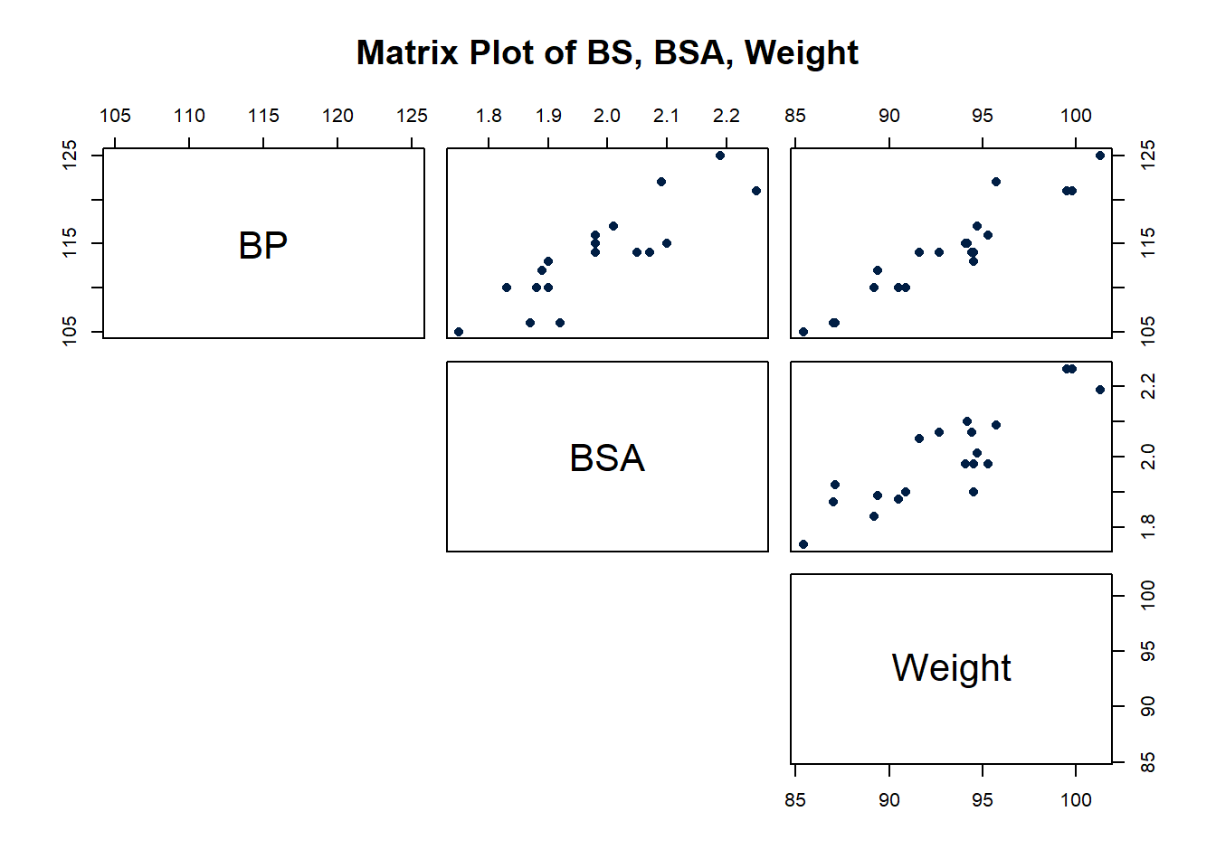
Scatterplot matrix plot of BP, BSA, Weight — Fig 12.5: Matrix Plot of BP, BSA, Weight

As the matrix plot and the following correlation matrix suggest:

Correlation: BP, Age, Weight, BSA, Dur, Pulse, Stress

	BP	Age	Weight	BSA	Dur
Age	0.659
Weight	0.950	0.407
BSA	0.866	0.378	0.875
Dur	0.293	0.344	0.201	0.131
Pulse	0.721	0.619	0.659	0.465	0.402
Stress	0.164	0.368	0.034	0.018	0.312

there appears to be not only a strong relationship between $y = BP$ and $x_2 = Weight$ ($r$ = 0.950) and a strong relationship between $y = BP$ and the predictor $x_3 = BSA$ ($r$ = 0.866), but also a strong relationship between the two predictors $x_2 = Weight$ and $x_3 = BSA$ ($r$ = 0.875). Incidentally, it shouldn’t be too surprising that a person’s weight and body surface area are highly correlated.

What impact does the strong correlation between the two predictors have on the regression analysis and the subsequent conclusions we can draw? Let’s proceed as before by reviewing the output of a series of regression analyses and collecting various pieces of information along the way. When we’re done, we’ll review what we learned by collating the various items in a summary table.

The regression of the response $y = BP$ on the predictor $x_2 = Weight$:

Analysis of Variance

Source	DF	Seq SS	Seq MS	F-Value	P-Value
Regression	1	505.472	505.472	166.86	0.000
Weight	1	505.472	505.472	166.86	0.000
Error	18	54.528	3.029
Lack-of-Fit	17	54.028	3.178	6.36	0.303
Pure Error	1	0.500	0.500
Total	19	560.00

Model Summary

S	R-sq	R-sq(adj)	R-sq(pred)
1.74050	90.23%	89.72%	88.53%

Coefficients

Term	Coef	SE Coef	T-Value	P-Value	VIF
Constant	2.21	8.66	0.25	0.802
Weight	1.2009	0.0930	12.92	0.000	1.00

Regression Equation

BP = 2.21 + 1.2009 Weight

yields the estimated coefficient $b_2$ = 1.2009, the standard error $se(b_2) = 0.0930$, and the regression sum of squares $SSR(x_2) = 505.472$.

The regression of the response $y = BP$ on the predictor $x_3 = BSA$:

Analysis of Variance

Source	DF	Seq SS	Seq MS	F-Value	P-Value
Regression	1	419.858	419.858	53.93	0.000
BSA	1	419.858	419.858	53.93	0.000
Error	18	140.142	7.786
Lack-of-Fit	13	133.642	10.280	7.91	0.016
Pure Error	5	6.500	1.300
Total	19	560.00

Model Summary

S	R-sq	R-sq(adj)	R-sq(pred)
2.79028	74.97%	73.58%	69.55%

Coefficients

Term	Coef	SE Coef	T-Value	P-Value	VIF
Constant	45.18	9.39	4.81	0.000

BSA	34.44	4.69	7.34	0.000	1.00

Regression Equation

BP = 45.18 + 34.44 BSA

yields the estimated coefficient $b_3$ = 34.44, the standard error $se(b_3) = 4.69$, and the regression sum of squares $SSR(x_3) = 419.858$.

The regression of the response $y = BP$ on the predictors $x_2 = Weight$ and $x_3 = BSA$ (in that order):

Analysis of Variance

Source	DF	Seq SS	Seq MS	F-Value	P-Value
Regression	2	508.286	254.143	83.54	0.000
Weight	1	505.472	505.472	166.16	0.000
BSA	1	2.814	2.814	0.93	0.350
Error	17	51.714	3.042
Total	19	560.00

Model Summary

S	R-sq	R-sq(adj)	R-sq(pred)
1.74413	90.77%	89.68%	87.78%

Coefficients

Term	Coef	SE Coef	T-Value	P-Value	VIF
Constant	5.65	9.39	0.60	0.555
Weight	1.039	0.193	5.39	0.000	4.28
BSA	5.83	6.06	0.96	0.350	4.28

Regression Equation

BP = 5.65 + 1.039 Weight + 5.83 BSA

yields the estimated coefficients $b_2$ = 1.039 and $b_3$ = 5.83, the standard errors $se(b_2) = 0.193$ and $se(b_3) = 6.06$, and the sequential sum of squares $SSR(x_3|x_2) = 2.814$.

And finally, the regression of the response $y = BP$ on the predictors $x_3 = BSA$ and $x_2 = Weight$ (in that order):

Analysis of Variance

Source	DF	Seq SS	Seq MS	F-Value	P-Value
Regression	2	508.29	254.143	83.54	0.000
BSA	1	419.86	419.858	138.02	0.000
Weight	1	88.43	88.428	29.07	0.000
Error	17	51.71	3.042
Total	19	560.00

Model Summary

S	R-sq	R-sq(adj)	R-sq(pred)
1.74413	90.77%	89.68%	87.78%

Coefficients

Term	Coef	SE Coef	T-Value	P-Value	VIF
Constant	5.65	9.39	0.60	0.555
BSA	5.83	6.06	0.96	0.350	4.28
Weight	1.039	0.193	5.39	0.000	4.28

Regression Equation

BP = 5.65 + 5.83 BSA + 1.039 Weight

yields the estimated coefficients $b_2$ = 1.039 and $b_3$ = 5.83, the standard errors $se(b_2) = 0.193$ and $se(b_3) = 6.06$, and the sequential sum of squares $SSR(x_2|x_3) = 88.43$.

Compiling the results in a summary table, we obtain:

Model	$b_2$	$se(b_2)$	$b_3$	$se(b_3)$	Seq SS
$x_2$ only	1.2009	0.0930	—	—	$SSR(x_2)$ 505.472
$x_3$ only	—	—	34.44	4.69	$SSR(x_3)$ 419.858
$x_2, x_3$ (in order)	1.039	0.193	5.83	6.06	$SSR(x_3 \mid x_2)$ 2.814
$x_3, x_2$ (in order)	1.039	0.193	5.83	6.06	$SSR(x_2 \mid x_3)$ 88.43

Geez — things look a little different than before. It appears as if, when predictors are highly correlated, the answers you get depend on the predictors in the model. That’s not good! Let’s proceed through the table and in so doing carefully summarize the effects of multicollinearity on the regression analyses.

Effect 1

When predictor variables are correlated, the estimated regression coefficient of any one variable depends on which other predictor variables are included in the model.

Here’s the relevant portion of the table:

Variables in model	$b_2$	$b_3$
$x_2$	1.20	—
$x_3$	—	34.4
$x_2,$ $x_3$	1.04	5.83

Note that, depending on which predictors we include in the model, we obtain wildly different estimates of the slope parameter for $x_3$ = BSA!

If $x_3 = BSA$ is the only predictor included in our model, we claim that for every additional one square meter increase in body surface area (BSA), blood pressure (BP) increases by 34.4 mm Hg.
On the other hand, if $x_2 = Weight$ and $x_3 = BSA$ are both included in our model, we claim that for every additional one square meter increase in body surface area (BSA), holding weight constant, blood pressure (BP) increases by only 5.83 mm Hg.

This is a huge difference! Our hope would be, of course, that two regression analyses wouldn’t lead us to such seemingly different scientific conclusions. The high correlation between the two predictors is what causes the large discrepancy. When interpreting $b_3$ = 34.4 in the model that excludes $x_2 = Weight$, keep in mind that when we increase $x_3 = BSA$ then $x_2 = Weight$ also increases and both factors are associated with increased blood pressure. However, when interpreting $b_3$ = 5.83 in the model that includes $x_2 = Weight$, we keep $x_2 = Weight$ fixed, so the resulting increase in blood pressure is much smaller.

The fantastic thing is that even predictors that are not included in the model, but are highly correlated with the predictors in our model, can have an impact! For example, consider a pharmaceutical company’s regression of territory sales on territory population and per capita income. One would, of course, expect that as the population of the territory increases, so would the sales in the territory. But, contrary to this expectation, the pharmaceutical company’s regression analysis deemed the estimated coefficient of territory population to be negative. That is, as the population of the territory increases, the territory sales were predicted to decrease. After further investigation, the pharmaceutical company determined that the larger the territory, the larger to the competitor’s market penetration. That is, the competitor kept the sales down in territories with large populations.

In summary, the competitor’s market penetration was not included in the original model. Yet, it was later deemed to be strongly positively correlated with territory population. Even though the competitor’s market penetration was not included in the original model, its strong correlation with one of the predictors in the model, greatly affected the conclusions arising from the regression analysis.

The moral of the story is that if you get estimated coefficients that just don’t make sense, there is probably a very good explanation. Rather than stopping your research and running off to report your unusual results, think long and hard about what might have caused the results. That is, think about the system you are studying and all of the extraneous variables that could influence the system.

Effect 2

When predictor variables are correlated, the precision of the estimated regression coefficients decreases as more predictor variables are added to the model.

Here’s the relevant portion of the table:

Variables in model	se($b_2$)	se($b_3$)
$x_2$	0.093	—
$x_3$	—	4.69
$x_2$, $x_3$	0.193	6.06

The standard error for the estimated slope $b_2$ obtained from the model including both $x_2 = Weight$ and $x_3 = BSA$ is about double the standard error for the estimated slope $b_2$ obtained from the model including only $x_2 = Weight$. And, the standard error for the estimated slope $b_3$ obtained from the model including both $x_2 = Weight$ and $x_3 = BSA$ is about 30% larger than the standard error for the estimated slope $b_3$ obtained from the model including only $x_3 = BSA$.

What is the major implication of these increased standard errors? Recall that the standard errors are used in the calculation of the confidence intervals for the slope parameters. That is, increased standard errors of the estimated slopes lead to wider confidence intervals and hence less precise estimates of the slope parameters.

Three plots to help clarify the second effect. Recall that the first Uncorrelated Predictors data set that we investigated in this lesson contained perfectly uncorrelated predictor variables ($r$ = 0). Upon regressing the response $y$ on the uncorrelated predictors $x_1$ and $x_2$, Minitab (or any other statistical software for that matter) will find the “best fitting” plane through the data points:

Fig 12.6: Interactive

Click the Best Fitting Plane button to see the best-fitting plane for this particular set of responses. Now, here’s where you have to turn on your imagination. The primary characteristic of the data — because the predictors are perfectly uncorrelated — is that the predictor values are spread out and anchored in each of the four corners, providing a solid base over which to draw the response plane. Now, even if the responses ($y$) varied somewhat from sample to sample, the plane couldn’t change all that much because of the solid base. That is, the estimated coefficients, $b_1$ and $b_2$ couldn’t change that much, and hence the standard errors of the estimated coefficients, $se(b_1)$ and $se(b_2)$ will necessarily be small.

Now, let’s take a look at the second example (bloodpress.txt) that we investigated in this lesson, in which the predictors $x_3 = BSA$ and $x_6 = Stress$ were nearly perfectly uncorrelated ($r$ = 0.018). Upon regressing the response $y = BP$ on the nearly uncorrelated predictors $x_3 = BSA$ and $x_6 = Stress$, we will again find the “best fitting” plane through the data points. Move the slider at the bottom of the graph to see the plane of best fit.

Fig 12.7: Interactive

Again, the primary characteristic of the data — because the predictors are nearly perfectly uncorrelated — is that the predictor values are spread out and just about anchored in each of the four corners, providing a solid base over which to draw the response plane. Again, even if the responses ($y$) varied somewhat from sample to sample, the plane couldn’t change all that much because of the solid base. That is, the estimated coefficients, $b_3$ and $b_6$ couldn’t change all that much. The standard errors of the estimated coefficients, $se(b_3)$ and $se(b_6)$, again will necessarily be small.

Now, let’s see what happens when the predictors are highly correlated. Let’s return to our most recent example (bloodpress.txt), in which the predictors $x_2 = Weight$ and $x_3 = BSA$ are very highly correlated ($r$ = 0.875). Upon regressing the response $y = BP$ on the predictors $x_2 = Weight$ and $x_3 = BSA$, Minitab will again find the “best fitting” plane through the data points.

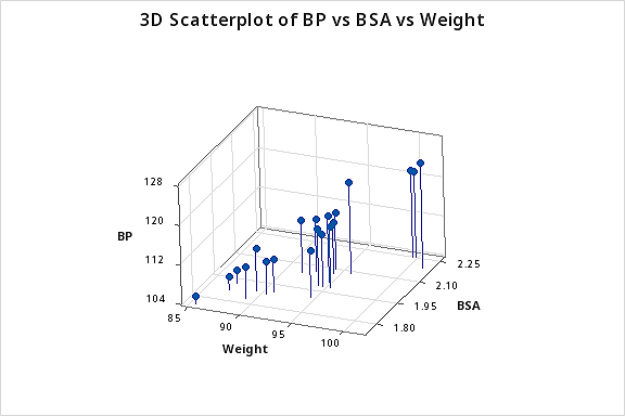
Fig 12.8: 3D Scatterplot of BP vs BSA vs Weight

Do you see the difficulty in finding the best-fitting plane in this situation? The primary characteristic of the data — because the predictors are so highly correlated — is that the predictor values tend to fall in a straight line. That is, there are no anchors in two of the four corners. Therefore, the base over which the response plane is drawn is not very solid.

Let’s put it this way — would you rather sit on a chair with four legs or one with just two legs? If the responses ($y$) varied somewhat from sample to sample, the position of the plane could change significantly. That is, the estimated coefficients, $b_2$ and $b_3$ could change substantially. The standard errors of the estimated coefficients, $se(b_2)$ and $se(b_3)$, will then be necessarily larger. Below is an animated view (no sound) of the problem that highly correlated predictors can cause with finding the best fitting plane.

Video 12.1: Effect of highly correlated predictors on best fitting planes

Effect 3

When predictor variables are correlated, the marginal contribution of any one predictor variable in reducing the error sum of squares varies depending on which other variables are already in the model.

For example, regressing the response $y = BP$ on the predictor $x_2 = Weight$, we obtain $SSR(x_2)$ = 505.472. But, regressing the response $y = BP$ on the two predictors $x_3 = BSA$ and $x_2 = Weight$ (in that order), we obtain $SSR(x_2|x_3)$ = 88.43. The first model suggests that weight reduces the error sum of squares substantially (by 505.472), but the second model suggests that weight doesn’t reduce the error sum of squares all that much (by 88.43) once a person’s body surface area is taken into account.

This should make intuitive sense. In essence, weight appears to explain some of the variations in blood pressure. However, because weight and body surface area are highly correlated, most of the variation in blood pressure explained by weight could just have easily been explained by body surface area. Therefore, once you take into account a person’s body surface area, there’s not much variation left in the blood pressure for weight to explain.

Incidentally, we see a similar phenomenon when we enter the predictors into the model in reverse order. That is, regressing the response $y = BP$ on the predictor $x_3 = BSA$, we obtain $SSR(x_3)$ = 419.858. But, regressing the response $y = BP$ on the two predictors $x_2 = Weight$ and $x_3 = BSA$ (in that order), we obtain $SSR(x_3|x_2)$ = 2.814. The first model suggests that body surface area reduces the error sum of squares substantially (by 419.858), and the second model suggests that body surface area doesn’t reduce the error sum of squares all that much (by only 2.814) once a person’s weight is taken into account.

Effect 4

When predictor variables are correlated, hypothesis tests for $\beta_k = 0$ may yield different conclusions depending on which predictor variables are in the model. (This effect is a direct consequence of the three previous effects.)

To illustrate this effect, let’s once again quickly proceed through the output of a series of regression analyses, focusing primarily on the outcome of the t-tests for testing $H_0 *{BSA} = 0 $ and $H_0* = 0 .$

The regression of the response $y= BP$ on the predictor $x_3 = BSA$:

Coefficients

Term	Coef	SE Coef	T-Value	P-Value	VIF
Constant	45.18	9.39	4.81	0.000
BSA	34.44	4.69	7.34	0.000	1.00

Regression Equation

BP = 45.18 + 34.44 BSA

indicates that the P-value associated with the t-test for testing $H_0 \colon \beta_{BSA} = 0$ is 0.000… < 0.01. There is sufficient evidence at the 0.05 level to conclude that blood pressure is significantly related to body surface area.

The regression of the response $y= BP$ on the predictor $x_2 = Weight$:

Coefficients

Term	Coef	SE Coef	T-Value	P-Value	VIF
Constant	2.21	8.66	0.25	0.802
Weight	1.2009	0.0930	12.92	0.000	1.00

Regression Equation

BP = 2.21 + 1.2009 Weight

indicates that the P-value associated with the t-test for testing $H_0 _{Weight} $ = 0 is 0.000… < 0.01. There is sufficient evidence at the 0.05 level to conclude that blood pressure is significantly related to weight.

And, the regression of the response $y= BP$ on the predictors $x_2 = Weight$ and $x_3 = BSA$:

Coefficients

Term	Coef	SE Coef	T-Value	P-Value	VIF
Constant	5.65	9.39	0.60	0.555
Weight	1.039	0.193	5.39	0.000	4.28
BSA	5.83	6.06	0.96	0.350	4.28

Regression Equation

BP = 112.72 + 0.0240 Stress

indicates that the P-value associated with the t-test for testing $H_0 \colon \beta_{Weight} = 0$ is 0.000… < 0.01. There is sufficient evidence at the 0.05 level to conclude that, after taking into account body surface area, blood pressure is significantly related to weight.

The regression also indicates that the P-value associated with the t-test for testing $H_0\colon\beta_{BSA} = 0$ is 0.350. There is insufficient evidence at the 0.05 level to conclude that blood pressure is significantly related to body surface area after taking into account weight. This might sound contradictory to what we claimed earlier, namely that blood pressure is indeed significantly related to body surface area. Again, what is going on here, once you take into account a person’s weight, body surface area doesn’t explain much of the remaining variability in blood pressure readings.

Effect 5

High multicollinearity among predictor variables does not prevent good, precise predictions of the response within the scope of the model.

Well, okay, it’s not an effect, and it’s not bad news either! It is good news! If the primary purpose of your regression analysis is to estimate a mean response $\mu_Y$ or to predict a new response $y$, you don’t have to worry much about multicollinearity.

For example, suppose you are interested in predicting the blood pressure ($y = BP$) of an individual whose weight is 92 kg and whose body surface area is 2 square meters:

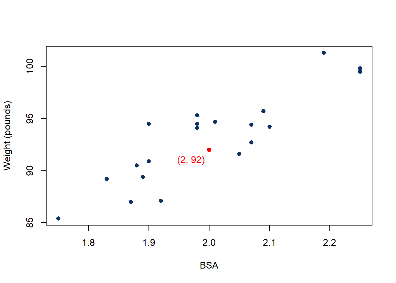
Scatterplot of Weight vs BSA (explanatory) in the bloodpress data. — Fig 12.9: Scatterplot of Weight vs BSA

Because point (2, 92) falls within the scope of the model, you’ll still get good, reliable predictions of the response $y$, regardless of the correlation that exists among the two predictors BSA and Weight. Geometrically, what is happening here is that the best-fitting plane through the responses may tilt from side to side from sample to sample (because of the correlation), but the center of the plane (in the scope of the model) won’t change all that much.

The following output illustrates how the predictions don’t change all that much from model to model:

Weight	Fit	SE Fit	95.0% CI	95.0% PI
92	112.7	0.402	(111.85, 113.54)	(108.94, 116.44)

BSA	Fit	SE Fit	95.0% CI	95.0% PI
2	114.1	0.624	(112.76, 115.38)	(108.06, 120.08)

BSA	Weight	Fit	SE Fit	95.0% CI	95.0% PI
2	92	112.8	0.448	(111.93, 113.83)	(109.08, 116.68)

The first output yields a predicted blood pressure of 112.7 mm Hg for a person whose weight is 92 kg based on the regression of blood pressure on weight. The second output yields a predicted blood pressure of 114.1 mm Hg for a person whose body surface area is 2 square meters based on the regression of blood pressure on body surface area. And the last output yields a predicted blood pressure of 112.8 mm Hg for a person whose body surface area is 2 square meters and whose weight is 92 kg based on the regression of blood pressure on body surface area and weight. Reviewing the confidence intervals and prediction intervals, you can see that they too yield similar results regardless of the model.

The bottom line

In short, what are the significant effects of multicollinearity on our use of a regression model to answer our research questions? In the presence of multicollinearity:

It is okay to use an estimated regression model to predict $y$ or estimate $\mu_Y$ as long as you do so within the model’s scope.
We can no longer make much sense of the usual interpretation of a slope coefficient as the change in the mean response for each additional unit increases in the predictor $x_k$ when all the other predictors are held constant.

The first point is, of course, addressed above. The second point is a direct consequence of the correlation among the predictors. It wouldn’t make sense to talk about holding the values of correlated predictors constant since changing one predictor necessarily would change the values of the others.

Try It! Correlated predictors

Effects of correlated predictor variables.

This exercise reviews the impacts of multicollinearity on various aspects of regression analyses. The Allen Cognitive Level (ACL) test is designed to quantify one’s cognitive abilities. David and Riley (1990) investigated the relationship of the ACL test to the level of psychopathology in a set of 69 patients from a general hospital psychiatry unit. The Allen Test data set contains the response $y$ = ACL and three potential predictors:

$x_1$ = Vocab, scores on the vocabulary component of the Shipley Institute of Living Scale
$x_2$ = Abstract, scores on the abstraction component of the Shipley Institute of Living Scale
$x_3$ = SDMT, scores on the Symbol-Digit Modalities Test

Determine the pairwise correlations among the predictor variables to get an idea of the extent to which the predictor variables are (pairwise) correlated. (See Minitab Help: Creating a correlation matrix). Also, create a matrix plot of the data to get a visual portrayal of the relationship between the response and predictor variables. (See Minitab Help: Creating a simple matrix of scatter plots)

Solution

There’s a moderate positive correlation between each pair of predictor variables, 0.698 for $X_1$ and $X_2,$ 0.556 for $X_1$ and $X_3,$ and 0.577 for $X_2$ and $X_3$

Fit the simple linear regression model with $y = ACL$ as the response and $x_1 = Vocab$ as the predictor. After fitting your model, request that Minitab predict the response $y = ACL$ when $x_1 = 25$. (See Minitab Help: Performing a multiple regression analysis — with options).
1. What is the value of the estimated slope coefficient $b_1$?
2. What is the value of the standard error of $b_1$?
3. What is the regression sum of squares, SSR ($x_1$), when $x_1$ is the only predictor in the model?
4. What is the predicted response of $y = ACL$ when $x_1 = 25$?

Solution

Estimated slope coefficient $b_1 = 0.0298$
Standard error $se(b_1) = 0.0141$
$SSR(X_1) = 2.691$
Predicted response when $x_1=25$ is 4.97025

Now, fit the simple linear regression model with $y = ACL$ as the response and $x_3 = SDMT$ as the predictor. After fitting your model, request that Minitab predict the response $y = ACL$ when $x_3$ = 40. (See Minitab Help: Performing a multiple regression analysis — with options).
1. What is the value of the estimated slope coefficient $b_3$?
2. What is the value of the standard error of $b_3$?
3. What is the regression sum of squares, SSR ($x_3$), when $x_3$ is the only predictor in the model?
4. What is the predicted response of $y = ACL$ when $x_3$ = 40?

Solution

Estimated slope coefficient $b_3 = 0.02807$
Standard error $se(b_3) = 0.00562$
$SSR(X_3) = 11.68$
Predicted response when $x_3=40$ is 4.87634

Fit the multiple linear regression model with $y = ACL$ as the response and $x_3 = SDMT$ as the first predictor and $x_1 = Vocab$ as the second predictor. After fitting your model, request that Minitab predict the response $y = ACL$ when $x_1$ = 25 and $x_3$ = 40. (See Minitab Help: Performing a multiple regression analysis — with options).
1. Now, what is the value of the estimated slope coefficient $b_1$? and $b_3$?
2. What is the value of the standard error of $b_1$? and $b_3$?
3. What is the sequential sum of squares, SSR ($X_1|X_3$?
4. What is the predicted response of $y = ACL$ when $x_1$ = 25 and $x_3$ = 40?

Solution

Estimated slope coefficient $b_1 = -0.0068$ (but not remotely significant) and $b_3 = 0.02979$
Standard error $se(b_1) = 0.0150$ and$se(b_3) = 0.00680$
$SSR(X_1|X_3) = 0.0979$
Predicted response when $x_1=25$ and $x_3=40$ is 4.86608

Summarize the effects of multicollinearity on various aspects of the regression analyses.

Solution

The regression output concerning $X_1=Vocab$ changes considerably depending on whether $X_3=SDMT$ is included or not. However, since $X_1$ is not remotely significant when $X_3$ is included, it is probably best to exclude $X_1$ from the model. The regression output concerning $X_3$ changes little depending on whether $X_1$ is included or not. Multicollinearity doesn’t have a particularly adverse effect in this example.

The regression output concerning $X_1=Vocab$ changes considerably depending on whether $X_3=SDMT$ is included or not. However, since $X_1$ is not remotely significant when $X_3$ is included, it is probably best to exclude $X_1$ from the model.The regression output concerning $X_3$ changes little depending on whether $X_1$ is included or not. Multicollinearity doesn’t have a particularly adverse effect in this example.

12.4 Detecting Multicollinearity Using Variance Inflation Factors

Okay, now that we know the effects that multicollinearity can have on our regression analyses and subsequent conclusions, how do we tell when it exists? That is, how can we tell if multicollinearity is present in our data?

Some of the common methods used for detecting multicollinearity include:

The analysis exhibits the signs of multicollinearity — such as estimates of the coefficients varying from model to model.
The t-tests for each of the individual slopes are non-significant (P > 0.05), but the overall F-test for testing all of the slopes is simultaneously 0 is significant (P < 0.05).
The correlations among pairs of predictor variables are large.

Looking at correlations only among pairs of predictors, however, is limiting. It is possible that the pairwise correlations are small, and yet a linear dependence exists among three or even more variables, for example, $X_3 = 2X_1 + 5X_2 + \text{error},$ say. That’s why many regression analysts often rely on what is called variance inflation factors (VIF) to help detect multicollinearity.

What is a Variation Inflation Factor?

As the name suggests, a variance inflation factor (VIF) quantifies how much the variance is inflated. But what variance? Recall that we learned previously that the standard errors — and hence the variances — of the estimated coefficients are inflated when multicollinearity exists. So, the variance inflation factor for the estimated coefficient $b_k$ — denoted $VIF_k$ — is just the factor by which the variance is inflated.

Let’s be a little more concrete. For the model in which $x_k$ is the only predictor:

\[y_i=\beta_0+\beta_kx_{ik}+\epsilon_i\]

it can be shown that the variance of the estimated coefficient $b_k$ is:

\[Var(b_k)_{min}=\dfrac{\sigma^2}{\sum_{i=1}^{n}(x_{ik}-\bar{x}_k)^2}\]

Note that we add the subscript “min” in order to denote that it is the smallest the variance can be. Don’t worry about how this variance is derived — we just need to keep track of this baseline variance, so we can see how much the variance of $b_k$ is inflated when we add correlated predictors to our regression model.

Let’s consider such a model with correlated predictors:

\[y_i=\beta_0+\beta_1x_{i1}+ \cdots + \beta_kx_{ik}+\cdots +\beta_{p-1}x_{i, p-1} +\epsilon_i\]

Now, again, if some of the predictors are correlated with the predictor $x_k,$ then the variance of $b_k$ is inflated. It can be shown that the variance of $b_k$ is:

\[Var(b_k)=\dfrac{\sigma^2}{\sum_{i=1}^{n}(x_{ik}-\bar{x}_k)^2}\times \dfrac{1}{1-R_{k}^{2}}\]

where $R_{k}^{2}$ is the $R^{2} \text{-value}$ obtained by regressing the $k^{th}$ predictor on the remaining predictors. Of course, the greater the linear dependence among the predictor $x_k$ and the other predictors, the larger the $R_{k}^{2}$ value. And, as the above formula suggests, the larger the $R_{k}^{2}$ value, the larger the variance of $b_k.$

How much larger? To answer this question, all we need to do is take the ratio of the two variances. By doing so, we obtain:

\[\dfrac{Var(b_k)}{Var(b_k)_{min}}=\dfrac{\left( \frac{\sigma^2}{\sum(x_{ik}-\bar{x}_k)^2}\times \dfrac{1}{1-R_{k}^{2}} \right)}{\left( \frac{\sigma^2}{\sum(x_{ik}-\bar{x}_k)^2} \right)}=\dfrac{1}{1-R_{k}^{2}}\]

The above quantity is deemed the variance inflation factor for the $k^{th}$ predictor. That is:

\[VIF_k=\dfrac{1}{1-R_{k}^{2}}\]

where $R_{k}^{2}$ is the $R^{2} \text{-value}$ obtained by regressing the $k^{th}$ predictor on the remaining predictors. Note that a variance inflation factor exists for each of the (p-1) predictors in a multiple regression model.

How do we interpret the variance inflation factors for a regression model? Again, it measures how much the variance of the estimated regression coefficient $b_k$ is “inflated” by the existence of correlation among the predictor variables in the model. A VIF of 1 means that there is no correlation between the $k^{th}$ predictor and the remaining predictor variables, and hence the variance of $b_k$ is not inflated at all. The general rule of thumb is that VIFs exceeding 4 further warrant investigation, while VIFs exceeding 10 are signs of serious multicollinearity requiring correction.

Example 12.2 (Continuing the Blood Pressure Data Set) Let’s return to the Blood Pressure data set in which researchers observed the following data on 20 individuals with high blood pressure:

blood pressure ($y = BP$, in mm Hg)
age ($x_{1}$ = Age, in years)
weight ($x_2 = Weight$, in kg)
body surface area ($x_{3}$ = BSA, in sq m)
duration of hypertension ($x_{4}$ = Dur, in years)
basal pulse ($x_{5}$ = Pulse, in beats per minute)
stress index ($x_{6}$ = Stress)

As you may recall, the matrix plot of BP, Age, Weight, and BSA:

the matrix plot of BP, Dur, Pulse, and Stress:

and the correlation matrix:

Correlation: BP, Age, Weight, BSA, Dur, Pulse, Stress

BP		Age	Weight	BSA	Due	Pulse
Age	0.659
Weight	0.950	0.407
BSA	0.866	0.378	0.875
Dur	0.293	0.344	0.201	0.131
Pulse	0.721	0.619	0.659	0.465	0.402
Stress	0.164	0.368	0.034	0.018	0.312	0.506

suggest that some of the predictors are at least moderately marginally correlated. For example, body surface area (BSA) and weight are strongly correlated ($r$ = 0.875), and weight and pulse are fairly strongly correlated ($r$ = 0.659). On the other hand, none of the pairwise correlations among age, weight, duration, and stress are particularly strong ($r$ < 0.40 in each case).

Regressing y = BP on all six of the predictors, we obtain:

Analysis of Variance

Source	DF	Seq SS	Seq MS	F-Value	P-Value
Regression	6	557.844	92.974	56.64	0.000
Age	1	243.266	243.266	1466.91	0.000
Weight	1	311.910	311.910	1880.84	0.000
BSA	1	1.768	1.768	10.66	0.006
Dur	1	0.335	0.335	2.02	0.179
Pulse	1	0.123	0.123	0.74	0.405
Stress	1	0.442	0.442	2.67	0.126
Error	13	2.156	0.166
Total	19	560.00

Model Summary

S	R-sq	R-sq(adj)	R-sq(pred)
0.407229	99.62%	99.44%	99.08%

Coefficients

Term	Coef	SE Coef	T-Value	P-Value	VIF
Constant	-12.87	2.56	-5.03	0.000
Age	0.7033	0.0496	14.18	0.000	1.76
Weight	0.9699	0.0631	15.37	0.000	8.42
BSA	3.78	1.58	2.39	0.033	5.33
Dur	0.0684	0.0484	1.41	0.182	1.24
Pulse	-0.0845	0.0516	-1.64	0.126	4.41
Stress	0.00557	0.00341	1.63	0.126	1.83

Minitab reports the variance inflation factors by default. As you can see, three of the variance inflation factors — 8.42, 5.33, and 4.41 — are fairly large. The VIF for the predictor Weight, for example, tells us that the variance of the estimated coefficient of Weight is inflated by a factor of 8.42 because Weight is highly correlated with at least one of the other predictors in the model.

For the sake of understanding, let’s verify the calculation of the VIF for the predictor Weight. Regressing the predictor $x_2 = Weight$ on the remaining five predictors:

Analysis of Variance

Source	DF	Seq SS	Seq MS	F-Value	P-Value
Regression	5	308.839	61.768	20.77	0.000
Age	1	15.04	15.04	0.50	0.490
BSA	1	212.734	212.734	71.53	0.000
Dur	1	1.442	1.442	0.48	0.498
Pulse	1	27.311	27.311	9.18	0.009
Stress	1	41.639	2.974
Error	14	41.639	2.974
Total	19	350.478

Model Summary

S	R-sq	R-sq(adj)	R-sq(pred)
1.72459	88.12%	83.88%	74.77%

Coefficients

Term	Coef	SE Coef	T-Value	P-Value	VIF
Constant	19.67	9.46	2.08	0.057
Age	-0.145	0.206	-0.70	0.495	1.70
BSA	21.42	3.46	6.18	0.000	1.43
Dur	0.009	0.205	0.04	0.967	1.24
Pulse	0.558	0.160	3.49	0.004	2.36
Stress	-0.0230	0.0131	-1.76	0.101	1.50

Minitab reports that $R_{Weight}^{2}$ is 88.1% or, in decimal form, 0.881. Therefore, the variance inflation factor for the estimated coefficient Weight is by definition:

\[VIF_{Weight}=\dfrac{Var(b_{Weight})}{Var(b_{Weight})_{min}}=\dfrac{1}{1-R_{Weight}^{2}}=\dfrac{1}{1-0.881}=8.4\]

Again, this variance inflation factor tells us that the variance of the weight coefficient is inflated by a factor of 8.4 because Weight is highly correlated with at least one of the other predictors in the model.

So, what to do? One solution to dealing with multicollinearity is to remove some of the violating predictors from the model. If we review the pairwise correlations again:

Correlation: BP, Age, Weight, BSA, Dur, Pulse, Stress

BP		Age	Weight	BSA	Dur	Pulse
Age	0.659
Weight	0.950	0.407
BSA	0.866	0.378	0.875
Dur	0.293	0.344	0.201	0.131
Pulse	0.721	0.619	0.659	0.465	0.402
Stress	0.164	0.368	0.034	0.018	0.312	0.506

we see that the predictors Weight and BSA are highly correlated ($r$ = 0.875). We can choose to remove either predictor from the model. The decision of which one to remove is often a scientific or practical one. For example, if the researchers here are interested in using their final model to predict the blood pressure of future individuals, their choice should be clear. Which of the two measurements — body surface area or weight — do you think would be easier to obtain?! If weight is an easier measurement to obtain than body surface area, then the researchers would be well-advised to remove BSA from the model and leave Weight in the model.

Reviewing again the above pairwise correlations, we see that the predictor Pulse also appears to exhibit fairly strong marginal correlations with several of the predictors, including Age ($r$ = 0.619), Weight ($r$ = 0.659), and Stress ($r$ = 0.506). Therefore, the researchers could also consider removing the predictor Pulse from the model.

Let’s see how the researchers would do. Regressing the response $y = BP$ on the four remaining predictors age, weight, duration, and stress, we obtain:

Analysis of Variance

Source	DF	Seq SS	Seq MS	F-Value	P-Value
Regression	4	555.455	138.864	458.28	0.000
Age	1	243.266	243.266	802.84	0.000
Weight	1	311.910	311.910	1029.38	0.000
Dur	1	0.178	0.178	0.59	0.455
Stress	1	0.100	0.100	0.33	0.573
Error	15	4.545	0.303
Total	19	560.000

Model Summary

S	R-sq	R-sq(adj)	R-sq(pred)
0.550462	99.19%	98.97%	98.59%

Coefficients

Term	Coef	SE Coef	T-Value	P-Value	VIF
Constant	-15.87	3.20	-4.97	0.000
Age	0.6837	0.0612	11.17	0.000	1.47
Weight	1.0341	0.0327	31.65	0.000	1.23
Dur	0.0399	0.0645	0.62	0.545	1.20
Stress	0.00218	0.00379	0.58	0.573	1.24

Aha — the remaining variance inflation factors are quite satisfactory! That is, it appears as if hardly any variance in inflation remains. Incidentally, in terms of the adjusted $R^{2} \text{-value},$ we did not seem to lose much by dropping the two predictors BSA and Pulse from our model. The adjusted $R^{2} \text{-value}$ decreased to only 98.97% from the original adjusted $R^{2} \text{-value}$ of 99.44%.

Video 12.2: Variance Inflation Factors

Try It! Variance inflation factors

Detecting multicollinearity using $VIF_k.$

We’ll use the Cement data set to explore variance inflation factors. The response y measures the heat evolved in calories during the hardening of cement on a per gram basis. The four predictors are the percentages of four ingredients: tricalcium aluminate ($x_{1}$), tricalcium silicate ($x_2$), tetracalcium alumino ferrite ($x_{3}$), and dicalcium silicate ($x_{4}$). It’s not hard to imagine that such predictors would be correlated in some way.

Use the Stat > Basic Statistics > Correlation … command in Minitab to get an idea of the extent to which the predictor variables are (pairwise) correlated. Also, use the Graph > Matrix Plot … command in Minitab to get a visual portrayal of the (pairwise) relationships among the response and predictor variables.

Solution

There’s a strong negative correlation between $X_2$ and $X_4$ (-0.973) and between $X_1$ and $X_3$ (-0.824). The remaining pairwise correlations are all quite low.

Regress the fourth predictor, $x_4$, on the remaining three predictors, $x_{1}$, $x_2$, and $x_{3}$. That is, fit the linear regression model treating $x_4$ as the response and $x_{1}$, $x_2,$ and $x_{3}$ as the predictors. What is the ${R^2}_4$ value? (Note that Minitab rounds the $R^{2}$ value it reports to three decimal places. For the purposes of the next question, you’ll want a more accurate $R^{2}$ value. Calculate the $R^{2}$ value SSR using its definition, $\dfrac{SSR}{SSTO}.$ Use your calculated value, carried out to 5 decimal places, in answering the next question.)

Solution

$R^2 = SSR/SSTO = 3350.10/3362.00 = 0.99646$

Using your calculated $R^{2}$ value carried out to 5 decimal places, determine by what factor the variance of $b_4$ is inflated. That is, what is $VIF_4$?

Solution

$VIF_4 = 1/(1-0.99646) - 282.5$

Minitab will actually calculate the variance inflation factors for you. Fit the multiple linear regression model with $y$ as the response and $x_{1},$$x_2,$$x_{3}$ and $x_{4}$ as the predictors. The $VIF_k$ will be reported as a column of the estimated coefficients table. Is the $VIF_4$ that you calculated consistent with what Minitab reports?

Solution

$VIF_4 = 282.51$

Note that all of the $VIF_k$ are larger than 10, suggesting that a high degree of multicollinearity is present. (It should seem logical that multicollinearity is present here, given that the predictors are measuring the percentage of ingredients in the cement.) Do you notice anything odd about the results of the t-tests for testing the individual $H_0\colon \beta_i = 0$ and the result of the overall F-test for testing $H_0\colon \beta_1 = \beta_2 = \beta_3 = \beta_4 = 0$? Why does this happen?

Solution

The individual t-tests indicate that none of the predictors are significant given the presence of all the others, but the overall F-test indicates that at least one of the predictors is useful. This is a result of the high degree of multicollinearity between all the predictors.

We learned that one way of reducing data-based multicollinearity is to remove some of the violating predictors from the model. Fit the linear regression model with y as the response and $X_1$ and $X_2$ as the only predictors. Are the variance inflation factors for this model acceptable?

Solution

The VIFs for the model with just $X_1$ and $X_2$ are just 1.06 and so are acceptable.

12.5 Reducing Data-based Multicollinearity

Recall that data-based multicollinearity is multicollinearity that results from a poorly designed experiment, reliance on purely observational data, or the inability to manipulate the system on which the data are collected. We now know all the bad things that can happen in the presence of multicollinearity. And, we’ve learned how to detect multicollinearity. Now, let’s learn how to reduce multicollinearity once we’ve discovered that it exists.

As the example in the previous section illustrated, one way of reducing data-based multicollinearity is to remove one or more of the violating predictors from the regression model. Another way is to collect additional data under different experimental or observational conditions. We’ll investigate this alternative method in this section.

Before we do, let’s quickly remind ourselves why we should care about reducing multicollinearity. It all comes down to drawing conclusions about the population slope parameters. If the variances of the estimated coefficients are inflated by multicollinearity, then our confidence intervals for the slope parameters are wider and therefore less useful. Eliminating or even reducing the multicollinearity, therefore, yields narrower, more useful confidence intervals for the slopes.

Example 12.3 (Allen Cognitive Level (ACL) Study) Researchers running the Allen Cognitive Level (ACL) Study were interested in the relationship of ACL test scores to the level of psychopathology. They, therefore, collected the following data on a set of 69 patients in a hospital psychiatry unit:

Response $y$ = ACL test score
Predictor $x_1$ = vocabulary (Vocab) score on the Shipley Institute of Living Scale
Predictor $x_2$ = abstraction (Abstract) score on the Shipley Institute of Living Scale
Predictor $x_3$ = score on the Symbol-Digit Modalities Test (SDMT)

For the sake of this example, I sampled 23 patients from the original data set in such a way as to ensure that a very high correlation exists between the two predictors Vocab and Abstract. A matrix plot of the resulting Allen Test n=23 data set:

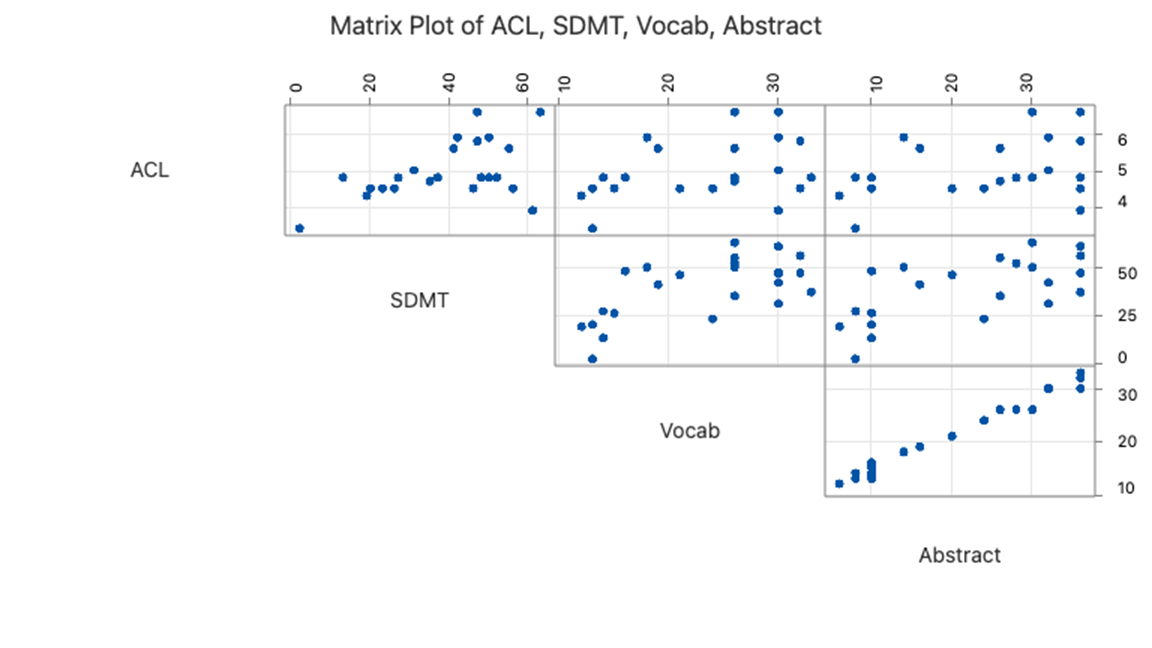
suggests that, indeed, a strong correlation exists between Vocab and Abstract. The correlations among the remaining pairs of predictors do not appear to be particularly strong.

Focusing only on the relationship between the two predictors Vocab and Abstract:

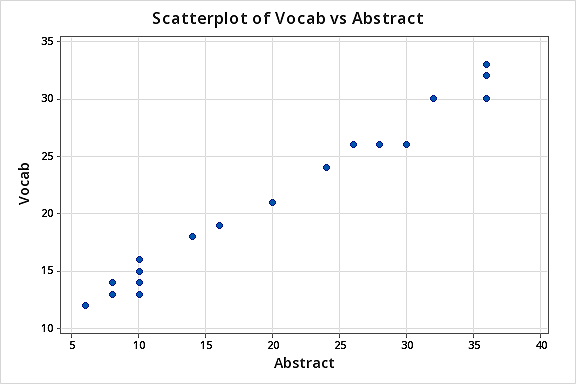
Pearson correlation of Vocab and Abstraction = 0.990

we do indeed see that a very strong relationship ($r$ = 0.99) exists between the two predictors.

Let’s see what havoc this high correlation wreaks on our regression analysis! Regressing the response $y = ACL$ on the predictors SDMT, Vocab, and Abstract, we obtain:

Analysis of Variance

Source	DF	Seq SS	Seq MS	F-Value	P-Value
Regression	3	3.6854	1.22847	2.28	0.112
SDMT	1	3.6346	3.63465	6.74	0.018
Vocab	1	0.0406	0.04064	0.08	0.787
Abstract	1	0.0101	0.01014	0.02	0.892
Error	19	10.2476	0.53935
Total	22	13.9330

Model Summary

S	R-sq	R-sq(adj)	R-sq(pred)
0.734404	26.45%	14.84%	0.00%

Coefficients

Term	Coef	SE Coef	T-Value	P-Value	VIF
Constant	3.75	1.34	2.79	0.012
SDMT	0.0233	0.0127	1.83	0.083	1.73
Vocab	0.028	0.152	0.19	0.855	49.29
Abstract	-0.014	0.101	-0.14	0.892	50.60

Yikes — the variance inflation factors for Vocab and Abstract are very large — 49.3 and 50.6, respectively!

What should we do about this? We could opt to remove one of the two predictors from the model. Alternatively, if we have a good scientific reason for needing both of the predictors to remain in the model, we could go out and collect more data. Let’s try this second approach here.

For the sake of this example, let’s imagine that we went out and collected more data, and in so doing, obtained the actual data collected on all 69 patients enrolled in the Allen Cognitive Level (ACL) Study. A matrix plot of the resulting Allen Test data set:

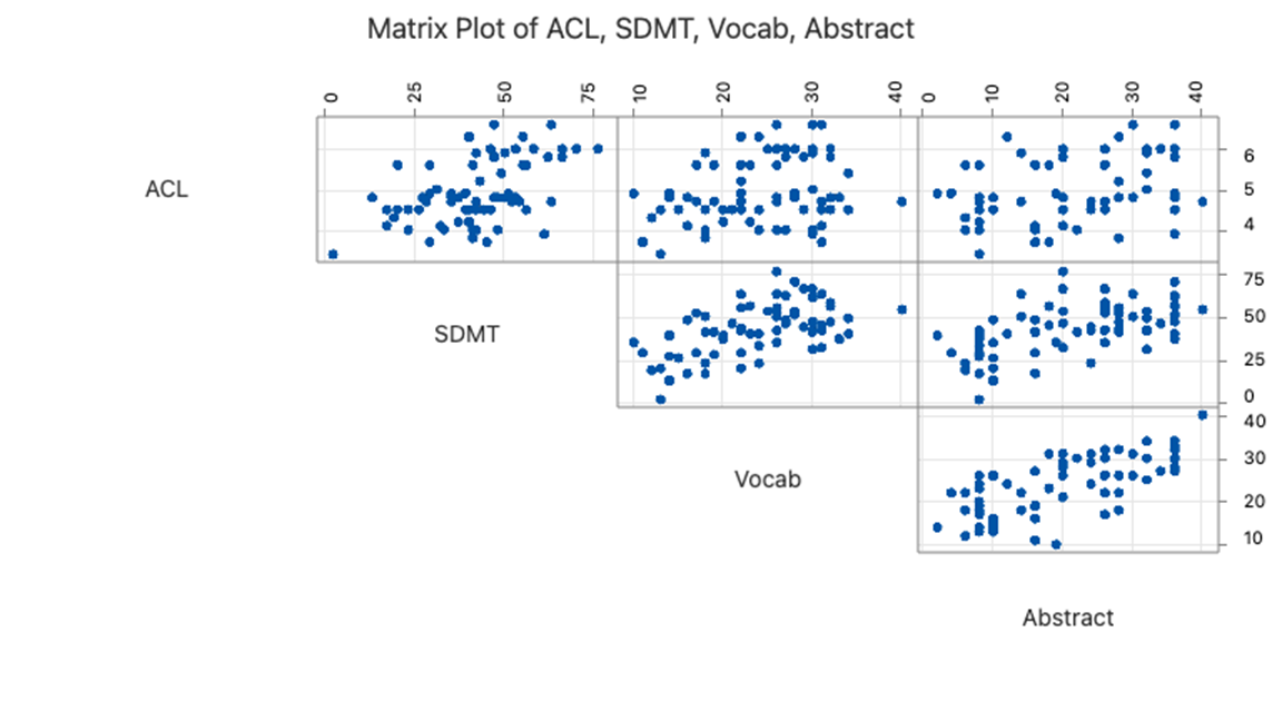
Pearson correlation of Vocab and Abstraction = 0.698

suggests that a correlation still exists between Vocab and Abstract — it is just a weaker correlation now.

Again, focusing only on the relationship between the two predictors Vocab and Abstract:

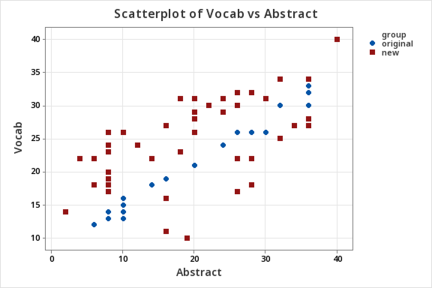
we do indeed see that the relationship between Abstract and Vocab is now much weaker ($r$ = 0.698) than before. The round data points in blue represent the 23 data points in the original data set, while the square red data points represent the 46 newly collected data points. As you can see from the plot, collecting the additional data has expanded the “base” over which the “best fitting plane” will sit. The existence of this larger base allows less room for the plane to tilt from sample to sample, and thereby reduces the variance of the estimated slope coefficients.

Let’s see if the addition of the new data helps to reduce the multicollinearity here. Regressing the response $y = ACL$ on the predictors SDMT, Vocab, and Abstract:

Analysis of Variance

Source	DF	Seq SS	Seq MS	F-Value	P-Value
Regression	3	12.3009	4.1003	8.67	0.000
SDMT	1	11.6799	11.6799	24.69	0.000
Vocab	1	0.0979	0.0979	0.21	0.651
Abstract	1	0.5230	0.5230	1.11	0.297
Error	65	30.7487	0.4731
Total	68	43.0496

Model Summary

S	R-sq	R-sq(adj)	R-sq(pred)
0.687791	28.57%	25.28%	19.93%

Coefficients

Term	Coef	SE Coef	T-Value	P-Value	VIF
Constant	3.946	0.338	11.67	0.000
SDMT	0.02740	0.00717	3.82	0.000	1.61
Vocab	-0.0174	0.0181	-0.96	0.339	2.09
Abstract	0.0122	0.0116	1.05	0.297	2.17

we find that the variance inflation factors are reduced significantly and satisfactorily. The researchers could now feel comfortable proceeding with drawing conclusions about the effects of the vocabulary and abstraction scores on the level of psychopathology.

Note!

One thing to keep in mind… In order to reduce the multicollinearity that exists, it is not sufficient to go out and just collect any old data. The data have to be collected in such a way as to ensure that the correlations among the violating predictors are actually reduced. That is, collecting more of the same kind of data won’t help to reduce the multicollinearity. The data have to be collected to ensure that the “base” is sufficiently enlarged. Doing so, of course, changes the characteristics of the studied population, and therefore should be reported accordingly.

12.6 Reducing Structural Multicollinearity

Recall that structural multicollinearity is multicollinearity that is a mathematical artifact caused by creating new predictors from other predictors, such as, creating the predictor $x^{2}$ from the predictor $x$. Because of this, at the same time that we learn here about reducing structural multicollinearity, we learn more about polynomial regression models.

Example 12.4 (Exercise and Immunity Study) What is the impact of exercise on the human immune system? To answer this very global and general research question, one has to first quantify what “exercise” means and what “immunity” means. Of course, there are several ways of doing so. For example, we might quantify one’s level of exercise by measuring his or her “maximal oxygen uptake.” And, we might quantify the quality of one’s immune system by measuring the amount of “immunoglobin in his or her blood.” In doing so, the general research question is translated into a much more specific research question: “How is the amount of immunoglobin in the blood ($y$) related to maximal oxygen uptake ($x$)?”

Because some researchers were interested in answering the above research question, they collected the following (Exercise and Immunity data set) on a sample of 30 individuals:

$y_i$ = amount of immunoglobin in the blood (mg) of individual $i$
$x_i$ = maximal oxygen uptake (ml/kg) of individual $i$

The scatter plot of the resulting data:

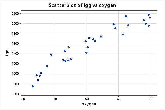
suggests that there might be some curvature to the trend in the data. To allow for the apparent curvature — rather than formulating a linear regression function — the researchers formulated the following quadratic (polynomial) regression function:

\[y_i=\beta_0+\beta_1x_i+\beta_{11}x_{i}^{2}+\epsilon_i\]

where:

$y_i$ = amount of immunoglobin in the blood (mg) of individual $i$
$x_i$ = maximal oxygen uptake (ml/kg) of individual $i$

As usual, the error terms $\epsilon_i$ are assumed to be independent, normally distributed, and have equal variance $\sigma^{2}$.

As the following plot of the estimated quadratic function suggests:

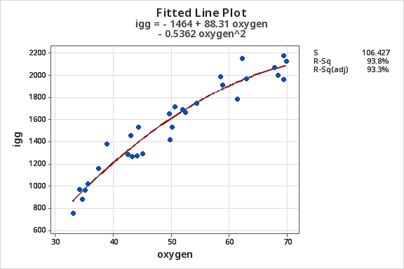
the formulated regression function appears to describe the trend in the data well. The adjusted $R^{2} \text{-value}$ is 93.3%.

But, now what do the estimated coefficients tell us? The interpretation of the regression coefficients is mostly geometric in nature. That is, the coefficients tell us a little bit about what the picture looks like:

If 0 is a possible $x$ value, then $b_0$ is the predicted response when $x$ = 0. Otherwise, the interpretation of $b_0$ is meaningless.
The estimated coefficient $b_1$ is the estimated slope of the tangent line at $x$ = 0.
The estimated coefficient $b_2$ indicates the up/down direction of the curve. That is:
- if $b_2$ < 0, then the curve is concave down
- if $b_2$ > 0, then the curve is concave up

So far, we have kept our heads a little bit in the sand! If we look at the output we obtain upon regressing the response y = igg on the predictors $\text{oxygen}$ and $\text{oxygen}^{2}$:

Analysis of Variance

Source	DF	Seq SS	Seq MS	F-Value	P-Value
Regression	2	4602211	2301105	203.16	0.000
oxygen	1	4472047	4472047	394.83	0.000
oxygensq	1	130164	130164	11.49	0.002
Error	27	305818	11327
Total	29	4908029

Model Summary

S	R-sq	R-sq(adj)	R-sq(pred)
106.427	93.77%	93.31%	92.48%

Coefficients

Term	Coef	SE Coef	T-Value	P-Value	VIF
Constant	-1464	411	-3.56	0.001
oxygen	88.3	16.5	5.36	0.000	99.94
oxygensq	-0.536	0.158	-3.39	0.002	99.94

we quickly see that the variance inflation factors for both predictors — oxygen, and oxygensq — are very large (99.9 in each case). Is this surprising to you? If you think about it, we’ve created a correlation by taking the predictor oxygen and squaring it to obtain oxygensq. That is, just by the nature of our model, we have created a “structural multicollinearity.”

The scatter plot of oxygensq versus oxygen:

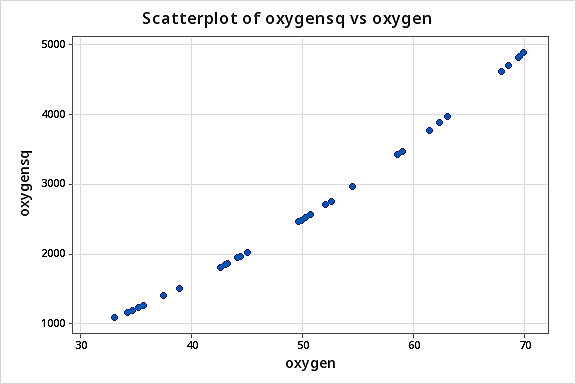
Pearson correlation of oxygen and oxygensq = 0.995

illustrates the intense strength of the correlation that we induced. After all, we just can’t get much more correlated than a correlation of $r$ = 0.995!

The neat thing here is that we can reduce the multicollinearity in our data by doing what is known as “centering the predictors.” Centering a predictor merely entails subtracting the mean of the predictor values in the data set from each predictor value. For example, Minitab reports that the mean of the oxygen values in our data set is 50.64:

Descriptive Statistics: oxygen

Variable	N	N*	Mean	SE Mean	StDev	Minimum	Q1	Median	Q3	Maximum
oxygen	30	0	50.64	2.19	11.99	33.00	41.58	50.00	61.63	69.90

Therefore, to center the predictor oxygen, we merely subtract 50.64 from each oxygen value in our data set. Doing so, we obtain the centered predictor, oxcent, say:

oxygen	oxcent	oxcentsq
34.6	-16.04	257.282
45.0	-5.64	31.810
62.3	11.66	135.956
58.9	8.26	68.228
42.5	-8.14	66.260
44.3	-6.34	40.196
67.9	17.26	297.908
58.5	7.86	61.780
35.6	-15.04	226.202
49.6	-1.04	1.082
33.0	-17.64	311.170

For example, 34.6 minus 50.64 is -16.04, and 45.0 minus 50.64 is -5.64, and so on. Now, to include the squared oxygen term in our regression model — to allow for curvature in the trend — we square the centered predictor oxcent to obtain oxcentsq. That is, $\left(-16.04\right)^{2} = 257.282$ and $\left(-5.64\right)^{2} = 31.810,$ and so on.

Wow! It really works! The scatter plot of oxcentsq versus oxcent:

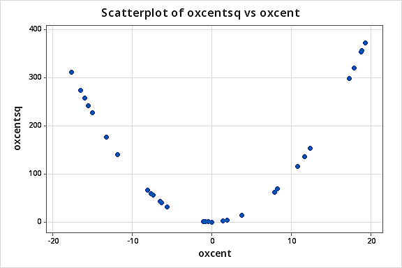
Pearson correlation of oxcent and oxygensq = 0.219

illustrates — by centering the predictors — just how much we’ve reduced the correlation between the predictor and its square. The correlation has gone from a whopping $r$ = 0.995 to a rather low $r$ = 0.219!

Having centered the predictor oxygen, we must reformulate our quadratic polynomial regression model accordingly. That is, we now formulate our model as:

\[y_i=\beta_{0}^{*}+\beta_{1}^{*}(x_i-\bar{x})+\beta_{11}^{*}(x_i-\bar{x})^{2}+\epsilon_i\]

or alternatively:

\[y_i=\beta_{0}^{*}+\beta_{1}^{*}x_{i}^{*}+\beta_{11}^{*}x_{i}^{*2}+\epsilon_i\]

where:

$y_i$ = amount of immunoglobin in the blood (mg), and
$x_{i}^{*}=x_i-\bar{x}$ denotes the centered predictor

and the error terms $\epsilon_i$ are independent, normally distributed and have equal variance $\sigma^{2}.$ Note that we add asterisks to each of the parameters to make it clear that the parameters differ from the parameters in the original model we formulated.

Let’s see how we did by centering the predictors and reformulating our model. Recall that — based on our original model — the variance inflation factors for oxygen and oxygensq were 99.9. Now, regressing y = igg on the centered predictors oxcent and oxcentsq:

Analysis of Variance

Source	DF	Seq SS	Seq MS	F-Value	P-Value
Regression	2	4602211	2301105	203.16	0.000
oxygen	1	4472047	4472047	394.83	0.000
oxygensq	1	130164	130164	11.49	0.002
Error	27	305818	11327
Total	29	4908029

Model Summary

S	R-sq	R-sq(adj)	R-sq(pred)
106.427	93.77%	93.31%	92.48%

Coefficients

Term	Coef	SE Coef	T-Value	P-Value	VIF
Constant	1632.3	29.3	55.62	0.000
oxygen	34.00	1.69	20.13	0.000	1.05
oxygensq	-0.536	0.158	-3.39	0.002	1.05

we see that the variance inflation factors have dropped significantly — now they are 1.05 in each case.

Because we reformulated our model based on the centered predictors, the meaning of the parameters must be changed accordingly. Now, the estimated coefficients tell us:

The estimated coefficient $b_0$ is the predicted response $y$ when the predictor $x$ equals the sample mean of the predictor values.
The estimated coefficient $b_1$ is the estimated slope of the tangent line at the predictor mean — and, often, it is similar to the estimated slope in the simple linear regression model.
The estimated coefficient $b_2$ indicates the up/down direction of the curve. That is:
- if $b_2$ < 0, then the curve is concave down
- if $b_2$ > 0, then the curve is concave up

So, here, in this example, the estimated coefficient $b_0$ = 1632.3 tells us that a male whose maximal oxygen uptake is 50.64 ml/kg is predicted to have 1632.3 mg of immunoglobin in his blood. And, the estimated coefficient $b_1$ = 34.00 tells us that when an individual’s maximal oxygen uptake is near 50.64 ml/kg, we can expect the individual’s immunoglobin to increase by 34.00 mg for every 1 ml/kg increase in maximal oxygen uptake.

As the following plot of the estimated quadratic function suggests:

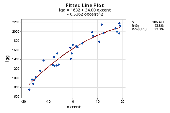
the reformulated regression function appears to describe the trend in the data well. The adjusted $R^{2} \text{-value}$ is still 93.3%.

We shouldn’t be surprised to see that the estimates of the coefficients in our reformulated polynomial regression model are quite similar to the estimates of the coefficients for the simple linear regression model:

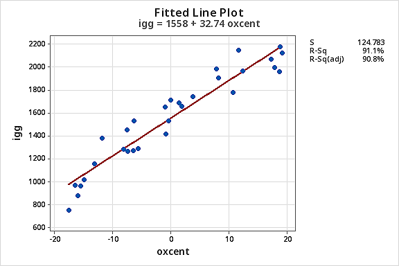
As you can see, the estimated coefficient $b_1$ = 34.00 for the polynomial regression model and $b_1$ = 32.74 for the simple linear regression model. And, the estimated coefficient $b_0$ = 1632 for the polynomial regression model and $b_0$ = 1558 for the simple linear regression model. The similarities in the estimates, of course, arise from the fact that the predictors are nearly uncorrelated and therefore the estimates of the coefficients don’t change all that much from model to model.

Now, you might be getting this sense that we’re “mucking around with the data” to get an answer to our research questions. One way to convince you that we’re not is to show you that the two estimated models are algebraically equivalent. That is, if given one form of the estimated model, say the estimated model with the centered predictors:

\[y_i=b_{0}^{*}+b_{1}^{*}x_{i}^{*}+b_{11}^{*}x_{i}^{*2}\]

then, the other form of the estimated model, say the estimated model with the original predictors:

\[y_i=b_{0}+b_{1}x_{i}+b_{11}x_{i}^{2}\]

can be easily obtained. In fact, it can be shown algebraically that the estimated coefficients of the original model equal:

\[\begin{align} b_{0}&=b_{0}^{*}-b_{1}^{*}\bar{x}+b_{11}^{*}\bar{x}^{2}\\ b_{1}&= b_{1}^{*}-2b_{11}^{*}\bar{x}\\ b_{11}&= b_{11}^{*}\\ \end{align}\]

For example, the estimated regression function for our reformulated model with centered predictors is:

\[\hat{y}_i=1632.3+34.00x_{i}^{*}-0.536x_{i}^{*2}\]

Then, since the mean of the oxygen values in the data set is 50.64:

Descriptive Statistics: oxygen

Variable	N	N*	Mean	SE Mean	StDev	Minimum	Q1	Median	Q3	Maximum
oxygen	30	0	50.64	2.19	11.99	33.00	41.58	50.00	61.63	69.90

it can be shown algebraically that the estimated coefficients for the model with the original (uncentered) predictors are:

$b_0 = 1632.3 - 34.00(50.64) - 0.536(50.64)^{2} = -1464$

$b_1 = 34.00 - 2(- 0.536)(50.64) = 88.3$

$b_{11} = - 0.536$

That is, the estimated regression function for our quadratic polynomial model with the original (uncentered) predictors is:

\[\hat{y}_i=-1464+88.3x_{i}-0.536x_{i}^{2}\]

Given the equivalence of the two estimated models, you might ask why we bother to center the predictors. The main reason for centering to correct structural multicollinearity is that low levels of multicollinearity can help avoid computational inaccuracies. Specifically, a near-zero determinant of $X^{T}X$ is a potential source of serious roundoff errors in the calculations of the normal equations. Severe multicollinearity has the effect of making this determinant come close to zero. Thus, under severe multicollinearity, the regression coefficients may be subject to large roundoff errors.

Let’s use our model to predict the immunoglobin level in the blood of a person whose maximal oxygen uptake is 90 ml/kg. Of course, before we use our model to answer a research question, we should always evaluate it first to make sure it means all of the necessary conditions. The residuals versus fits plot:

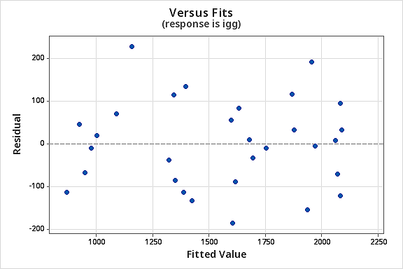
shows a nice horizontal band around the residual = 0 line, suggesting the model fits the data well. It also suggests that the variances of the error terms are equal. And, the normal probability plot:

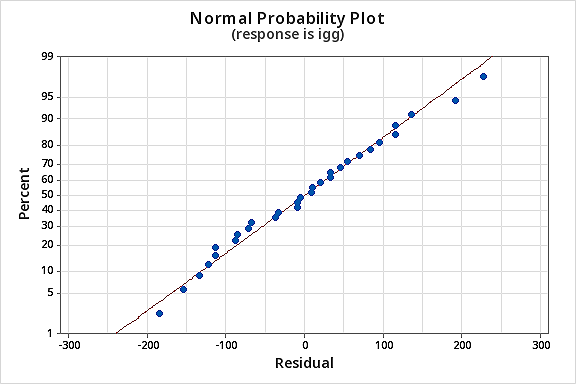
suggests that the error terms are normally distributed. Okay, we’re good to go — let’s use the model to answer our research question: “What is one’s predicted IgG if the maximal oxygen uptake is 90 ml/kg?”

When asking Minitab to make this prediction, you have to remember that we have centered the predictors. That is, if oxygen = 90, then oxcent = 90-50.64 = 39.36. And, if oxcent = 39.36, then oxcentsq = 1549.210. Asking Minitab to predict the igg of an individual whose oxcent = 39.4 and oxcentsq = 1549, we obtain the following output:

Regression Equation

igg = 1632.3 + 34.00 oxcent - 0.536 oxcentsq

variable	Setting
oxcent	39.4
oxcentsq	1549

Fit	SE Fit	95% CI	95% PI
2141.10	219.209	(1691.32, 2590.88)	(1641.12, 2641.09)	XX

XX denotes an extremely unusual point relative to predictor levels used to fit the model

Why does Minitab report that “XX denotes a row with very extreme X values?” Recall that the levels of maximal oxygen uptake in the data set ranged from 30 to 70 ml/kg. Therefore, a maximal oxygen uptake of 90 is way outside the scope of the model, and Minitab provides such a warning.

A word of warning. Be careful — because of changes in direction of the curve, there is an even greater danger of extrapolation when modeling data with a polynomial function.

The hierarchical approach to model fitting

Just one closing comment since we’ve been discussing polynomial regression to remind you about the “hierarchical approach to model fitting.” The widely accepted approach to fitting polynomial regression functions is to fit a higher-order model and then explore whether a lower-order (simpler) model is adequate. For example, suppose we formulate the following cubic polynomial regression function:

\[y_i=\beta_{0}+\beta_{1}x_{i}+\beta_{11}x_{i}^{2}+\beta_{111}x_{i}^{3}+\epsilon_i\]

Then, to see if the simpler first-order model (a “line”) is adequate in describing the trend in the data, we could test the null hypothesis:

\[H_0 \colon \beta_{11}=\beta_{111}=0\]

But then … if a polynomial term of a given order is retained, then all related lower-order terms are also retained. That is, if a quadratic term is deemed significant, then it is standard practice to use this regression function:

\[\mu_Y=\beta_{0}+\beta_{1}x_{i}+\beta_{11}x_{i}^{2}\]

and not this one:

\[\mu_Y=\beta_{0}+\beta_{11}x_{i}^{2}\]

That is, we always fit the terms of a polynomial model in a hierarchical manner.

12.7 Further Example

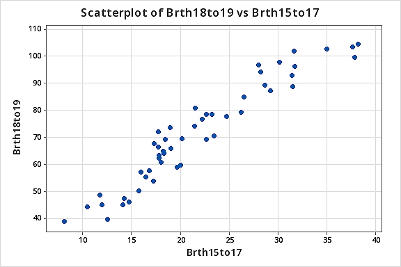
Example 12.5 (Poverty and Teen Birth Rate Data) (Data source: The U.S. Census Bureau and Mind On Statistics, (3rd edition), Utts and Heckard). In this example, the observations are the 50 states of the United States (Poverty data) - Note: remove data from the District of Columbia). The variables are $y$ = percentage of each state’s population living in households with income below the federally defined poverty level in the year 2002, $x_{1}$ = birth rate for females 15 to 17 years old in 2002, calculated as births per 1000 persons in the age group, and $x_{2}$ = birth rate for females 18 to 19 years old in 2002, calculated as births per 1000 persons in the age group.

The two $x$-variables are correlated (so we have multicollinearity). The correlation is about 0.95. A plot of the two $x$-variables is given below.

The figure below shows plots of $y$ = poverty percentage versus each $x$-variable separately. Both $x$-variables are linear predictors of the poverty percentage.

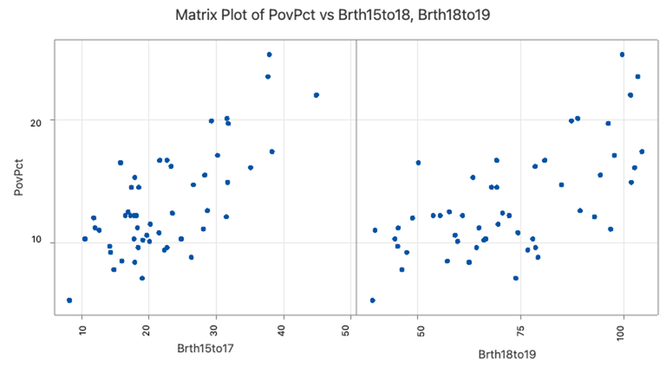
Minitab results for the two possible simple regressions and the multiple regression are given below.

Regression Analysis: PovPct versus Brth15to17

Regression Equation

PovPct = 4.49 + 0.387 Brth15to17

Predictor	Coef	SE Coef	T	P
Constant	4.487	1.318	3.40	0.001
Brth15to17	0.38718	0.05720	6.77	0.000

S = 2.98209 R-Sq = 48.8% R-Sq(adj) = 47.8%

Regression Analysis: PovPct versus Brth18to19

Regression Equation

PovPct = 3.05 + 0.138 Brth18to19

Predictor	Coef	SE Coef	T	P
Constant	3.053	1.832	1.67	0.102
Brth18to19	0.13842	0.02482	5.58	0.000

S = 3.24777 R-Sq = 39.3% R-Sq(adj) = 38.0%

Regression Analysis: PovPct versus Brth15to17, Brth18to19

Regression Equation

PovPct = 6.44 + 0.632 Brth15to17 - 0.102 Brth18to19

Predictor	Coef	SE Coef	T	P
Constant	6.440	1.959	3.29	0.002
Brth15to17	0.6323	0.1918	3.30	0.002
Brth18to19	-0.10227	0.07642	-1.34	0.187

s = 2.95782 R-Sq = 50.7% R-Sq(adj) = 48.6%

We note the following:

The value of the sample coefficient that multiplies a particular $x$-variable is not the same in the multiple regression as it is in the relevant simple regression.
The $R^{2}$ for the multiple regression is not the sum of the $R^{2}$ values for the simple regressions. An $x$-variable (either one) is not making an independent “add-on” in the multiple regression.
The 18 to 19-year-old birth rate variable is significant in the simple regression but is not in the multiple regression. This discrepancy is caused by the correlation between the two $x$-variables. The 15 to 17-year-old birth rate is the stronger of the two $x$-variables and given its presence in the equation, the 18 to 19-year-old rate does not improve $R^{2}$ enough to be significant. More specifically, the correlation between the two x-variables has increased the standard errors of the coefficients, so we have less precise estimates of the individual slopes.

12.8 Extrapolation

“Extrapolation” beyond the “scope of the model” occurs when one uses an estimated regression equation to estimate a mean $\mu_{Y}$ or to predict a new response $y_{new}$ for $x$ values not in the range of the sample data used to determine the estimated regression equation. In general, it is dangerous to extrapolate beyond the scope of the model. The following example illustrates why this is not a good thing to do.

Researchers measured the number of colonies of grown bacteria for various concentrations of urine (ml/plate). The scope of the model — that is, the range of the $x$ values — was 0 to 5.80 ml/plate. The researchers obtained the following estimated regression equation:

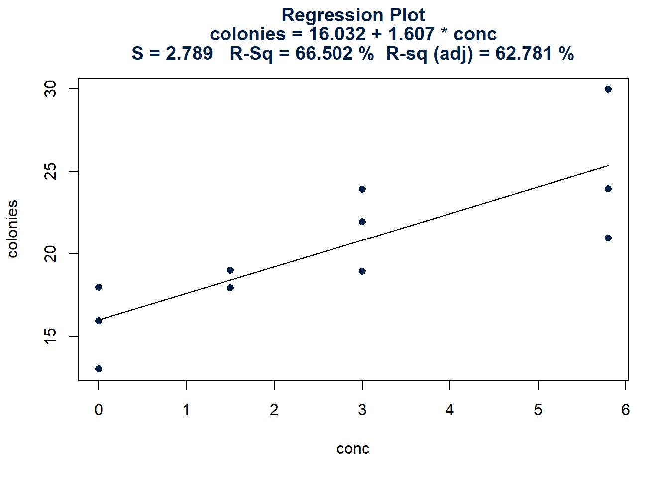
Fig 12.26: Colonies vs Concentrations Regression plot

Using the estimated regression equation, the researchers predicted the number of colonies at 11.60 ml/plate to be 16.032 + 1.1.607(11.60) or 34.6732 colonies. But when the researchers conducted the experiment at 11.60 ml/plate, they observed that the number of colonies decreased dramatically to about 15.1 ml/plate:

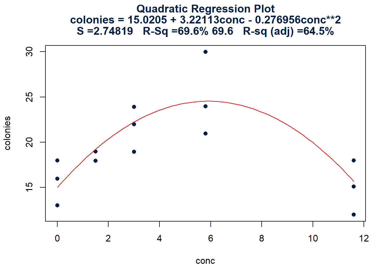
Colonies vs Concentrations Regression plot with a quadratic fit — Fig 12.27: Colonies vs Concentrations Regression plot (Quadratic)

The moral of the story is that the trend in the data as summarized by the estimated regression equation does not necessarily hold outside the scope of the model.

12.9 Other Regression Pitfalls

Nonconstant Variance

Excessive nonconstant variance can create technical difficulties with a multiple linear regression model. For example, if the residual variance increases with the fitted values, then prediction intervals will tend to be wider than they should be at low fitted values and narrower than they should be at high fitted values. Some remedies for refining a model exhibiting excessive nonconstant variance include the following:

Apply a variance-stabilizing transformation to the response variable, for example, a logarithmic transformation (or a square root transformation if a logarithmic transformation is “too strong” or a reciprocal transformation if a logarithmic transformation is “too weak”). We explored this in more detail in Lesson 9.
Weight the variances so that they can be different for each set of predictor values. This leads to weighted least squares, in which the data observations are given different weights when estimating the model. We’ll cover this in Lesson 13.
A generalization of weighted least squares is to allow the regression errors to be correlated with one another in addition to having different variances. This leads to generalized least squares, in which various forms of nonconstant variance can be modeled.
For some applications, we can explicitly model the variance as a function of the mean, $E(Y)$. This approach uses the framework of generalized linear models, which we discuss in the optional content.

Autocorrelation

One common way for the “independence” condition in a multiple linear regression model to fail is when the sample data have been collected over time and the regression model fails to effectively capture any time trends. In such a circumstance, the random errors in the model are often positively correlated over time, so each random error is more likely to be similar to the previous random error than it would be if the random errors were independent of one another. This phenomenon is known as autocorrelation (or serial correlation) and can sometimes be detected by plotting the model residuals versus time. We’ll explore this further in the optional content.

Overfitting

When building a regression model, we don’t want to include unimportant or irrelevant predictors whose presence can overcomplicate the model and increase our uncertainty about the magnitudes of the effects for the important predictors (particularly if some of those predictors are highly collinear). Such “overfitting” can occur the more complicated a model becomes and the more predictor variables, transformations, and interactions are added to a model. It is always prudent to apply a sanity check to any model being used to make decisions. Models should always make sense, preferably grounded in some kind of background theory or sensible expectation about the types of associations allowed between variables. Predictions from the model should also be reasonable (over-complicated models can give quirky results that may not reflect reality).

Excluding Important Predictor Variables

However, there is a potentially greater risk from excluding important predictors than from including unimportant ones. The linear association between two variables ignoring other relevant variables can differ both in magnitude and direction from the association that controls for other relevant variables. Whereas the potential cost of including unimportant predictors might be increased difficulty with interpretation and reduced prediction accuracy, the potential cost of excluding important predictors can be a completely meaningless model containing misleading associations. Results can vary considerably depending on whether such predictors are (inappropriately) excluded or (appropriately) included. These predictors are sometimes called confounding or lurking variables, and their absence from a model can lead to incorrect decisions and poor decision-making.

Example 12.6 (Simpson’s Paradox) An illustration of how a response variable can be positively associated with one predictor variable when ignoring a second predictor variable, but negatively associated with the first predictor when controlling for the second predictor. The dataset used in the example is available in this file: paradox.txt.

Video 12.3: Simpson’s Paradox

Missing Data

Real-world datasets frequently contain missing values, so we do not know the values of particular variables for some of the sample observations. For example, such values may be missing because they were impossible to obtain during data collection. Dealing with missing data is a challenging task. Missing data has the potential to adversely affect a regression analysis by reducing the total usable sample size. The best solution to this problem is to try extremely hard to avoid missing data in the first place. When there are missing values that are impossible or too costly to avoid, one approach is to replace the missing values with plausible estimates, known as imputation. Another (easier) approach is to consider only models that contain predictors with no (or few) missing values. This may be unsatisfactory, however, because even a predictor variable with a large number of missing values can contain useful information.

Power and Sample Size

In small datasets, a lack of observations can lead to poorly estimated models with large standard errors. Such models are said to lack statistical power because there is insufficient data to be able to detect significant associations between the response and predictors. So, how much data do we need to conduct a successful regression analysis? A common rule of thumb is that 10 data observations per predictor variable are a pragmatic lower bound for sample size. However, it is not so much the number of data observations that determines whether a regression model is going to be useful, but rather whether the resulting model satisfies the LINE conditions. In some circumstances, a model applied to fewer than 10 data observations per predictor variable might be perfectly fine (if, say, the model fits the data really well and the LINE conditions seem fine), while in other circumstances a model applied to a few hundred data points per predictor variable might be pretty poor (if, say, the model fits the data badly and one or more conditions are seriously violated). For another example, in general, we’d need more data to model interaction compared to a similar model without the interaction. However, it is difficult to say exactly how much data would be needed. It is possible that we could adequately model interaction with a relatively small number of observations if the interaction effect was pronounced and there was little statistical error. Conversely, in datasets with only weak interaction effects and relatively large statistical errors, it might take a much larger number of observations to have a satisfactory model. In practice, we have methods for assessing the LINE conditions, so it is possible to consider whether an interaction model approximately satisfies the assumptions on a case-by-case basis. In conclusion, there is not really a good standard for determining sample size given the number of predictors, since the only truthful answer is, “It depends.” In many cases, it soon becomes pretty clear when working on a particular dataset if we are trying to fit a model with too many predictor terms for the number of sample observations (results can start to get a little odd, and standard errors greatly increase). From a different perspective, if we are designing a study and need to know how much data to collect, then we need to get into sample size and power calculations, which rapidly become quite complex. Some statistical software packages will do sample size and power calculations, and there is even some software specifically designed to do just that. When designing a large, expensive study, it is recommended that such software be used or get advice from a statistician with sample size expertise.

Software Help 12

The next sections cover the Minitab and R commands for the procedures in this lesson.

Minitab Help 12: Multicollinearity

Blood pressure (predictors with high multicollinearity)

Create a simple matrix of scatterplots of the data.
Perform a linear regression analysis of BP vs Weight.
Perform a linear regression analysis of BP vs BSA.
Perform a linear regression analysis of BP vs Weight + BSA.
Perform a linear regression analysis of BP vs BSA + Weight.
Select Graph > 3D Scatterplot to create a 3D scatterplot of the data.
Find a confidence interval and a prediction interval for the response to predict BP for Weight=92 and BSA=2 for the two simple linear regression models and the multiple linear regression model.

Poverty and teen birth rate (high multicollinearity)

Select Data > Subset Worksheet to create a worksheet that excludes the District of Columbia.
Create a simple matrix of scatterplots of the data.
Perform a linear regression analysis of PovPct vs Brth15to17.
Perform a linear regression analysis of PovPct vs Brth18to19.
Perform a linear regression analysis of PovPct vs Brth15to17 + Brth18to19.

Blood pressure (high multicollinearity)

Perform a linear regression analysis of BP vs Age + Weight + BSA + Dur + Pulse + Stress.
Perform a linear regression analysis of Weight vs Age + BSA + Dur + Pulse + Stress and confirm the VIF value for Weight as 1/(1-R²) for this model.
Perform a linear regression analysis of BP vs Age + Weight + Dur + Stress.

Allen Cognitive Level study (reducing data-based multicollinearity)

Create a simple matrix of scatterplots of the sampled allentestn23 data.
Obtain a sample correlation between Vocab and Abstract.
Perform a linear regression analysis of ACL vs SDMT + Vocab + Abstract.
Repeat for the full allentest data.

Exercise and immunity (reducing structural multicollinearity)

Create a basic scatterplot of igg vs oxygen.
Select Calc > Calculator to calculate an oxygen-squared variable named oxygensq.
Perform a linear regression analysis of igg vs oxygen + oxygensq.
Create a fitted line plot and select “Quadratic” for the type of regression model.
Create a basic scatterplot of oxygensq vs oxygen.
Obtain a sample correlation between oxygensq and oxygen.
Select Calc > Calculator to calculate a centered oxygen variable named oxcent and an oxcent-squared variable named oxcentsq.
Perform a linear regression analysis of igg vs oxcent + oxcentsq.
Create a fitted line plot and select “Quadratic” for the type of regression model.
Perform a linear regression analysis of igg vs oxcent.
Create residual plots to create a residual vs fits plot and a normal probability plot for the centered quadratic model.
Find a confidence interval and a prediction interval for the response to predict igg for oxygen = 70 using the centered quadratic model.

R Help 12: Multicollinearity

The R logo

Blood pressure (multicollinearity)

Load the bloodpress data.
Create scatterplot matrices of the data.
Calculate correlations between the variables.

Show the codebloodpress <- read.table("Data_files/bloodpress.txt", header=T)
attach(bloodpress)

pairs(bloodpress[,c(2:5)])
pairs(bloodpress[,c(2,6:8)])

round(cor(bloodpress[,c(2:8)]),3)

detach(bloodpress)

Uncorrelated predictors (no multicollinearity)

Load the uncorrpreds data.
Create a scatterplot matrix of the data.
Calculate the correlation between the predictors.
Fit a simple linear regression model of y vs $x_1.$
Fit a simple linear regression model of y vs $x_2.$
Fit a multiple linear regression model of y vs $x_1$ + $x_2.$
Fit a multiple linear regression model of y vs $x_2$ + $x_1.$
Use the scatter3d function in the car package to create a 3D scatterplot of the data with the fitted plane for a multiple linear regression model of y vs $x_1$ + $x_2.$

Show the codeuncorrpreds <- read.table("Data_files/uncorrpreds.txt", header=T)
attach(uncorrpreds)

pairs(uncorrpreds)

cor(x1,x2) 

model.1 <- lm(y ~ x1)
summary(model.1)

anova(model.1)

model.2 <- lm(y ~ x2)
summary(model.2)

anova(model.2)

model.12 <- lm(y ~ x1 + x2)
summary(model.12)

anova(model.12)

model.21 <- lm(y ~ x2 + x1)
summary(model.21)

anova(model.21)

library(car)
scatter3d(y ~ x1 + x2)

detach(uncorrpreds)

Blood pressure (predictors with almost no multicollinearity)

Load the bloodpress data.
Create a scatterplot matrix of the data.
Fit a simple linear regression model of BP vs Stress.
Fit a simple linear regression model of BP vs BSA.
Fit a multiple linear regression model of BP vs Stress + BSA.
Fit a multiple linear regression model of BP vs BSA + Stress.
Use the scatter3d function in the car package to create a 3D scatterplot of the data with the fitted plane for a multiple linear regression model of BP vs Stress + BSA.

Show the codeattach(bloodpress)

pairs(bloodpress[,c(2,5,8)])

model.1 <- lm(BP ~ Stress)
summary(model.1)

anova(model.1)

model.2 <- lm(BP ~ BSA)
summary(model.2)

anova(model.2)

model.12 <- lm(BP ~ Stress + BSA)
summary(model.12)

anova(model.12)

model.21 <- lm(BP ~ BSA + Stress)
summary(model.21)

anova(model.21)

scatter3d(BP ~ Stress + BSA)

detach(bloodpress)

Blood pressure (predictors with high multicollinearity)

Load the bloodpress data.
Create a scatterplot matrix of the data.
Fit a simple linear regression model of BP vs Weight.
Fit a simple linear regression model of BP vs BSA.
Fit a multiple linear regression model of BP vs Weight + BSA.
Fit a multiple linear regression model of BP vs BSA + Weight.
Use the scatter3d function in the car package to create a 3D scatterplot of the data with the fitted plane for a multiple linear regression model of BP vs Weight + BSA.
Predict BP for Weight=92 and BSA=2 for the two simple linear regression models and the multiple linear regression model.

Show the codeattach(bloodpress)

pairs(bloodpress[,c(2,5,4)])

model.1 <- lm(BP ~ Weight)
summary(model.1)

anova(model.1)

model.2 <- lm(BP ~ BSA)
summary(model.2)

model.12 <- lm(BP ~ Weight + BSA)
summary(model.12)

model.21 <- lm(BP ~ BSA + Weight)
summary(model.21)

anova(model.21)

scatter3d(BP ~ Weight + BSA)

predict(model.1, interval="prediction",
        newdata=data.frame(Weight=92))

predict(model.2, interval="prediction",
        newdata=data.frame(BSA=2))

predict(model.12, interval="prediction",
        newdata=data.frame(Weight=92, BSA=2))

detach(bloodpress)

Poverty and teen birth rate (high multicollinearity)

Load the poverty data and remove the District of Columbia.
Create a scatterplot matrix of the data.
Fit a simple linear regression model of PovPct vs Brth15to17.
Fit a simple linear regression model of PovPct vs Brth18to19.
Fit a multiple linear regression model of PovPct vs Brth15to17 + Brth18to19.

Show the codepoverty <- read.table("Data_files/poverty.txt", header=T)
poverty <- poverty[poverty$Location!="District_of_Columbia",]
attach(poverty)

pairs(poverty[,c(2:4)])

model.1 <- lm(PovPct ~ Brth15to17)
summary(model.1)

model.2 <- lm(PovPct ~ Brth18to19)
summary(model.2)

model.12 <- lm(PovPct ~ Brth15to17 + Brth18to19)
summary(model.12)

detach(poverty)

Blood pressure (high multicollinearity)

Load the bloodpress data.
Fit a multiple linear regression model of BP vs Age + Weight + BSA + Dur + Pulse + Stress.
Use the vif function in the car package to calculate variance inflation factors.
Fit a multiple linear regression model of Weight vs Age + BSA + Dur + Pulse + Stress and confirm the VIF value for Weight as 1/(1-$R^2$) for this model.
Fit a multiple linear regression model of BP vs Age + Weight + Dur + Stress.
Use the vif function in the car package to calculate variance inflation factors.

Show the codeattach(bloodpress)

model.1 <- lm(BP ~ Age + Weight + BSA + Dur + Pulse + Stress)
summary(model.1)

library(car)
vif(model.1)

model.2 <- lm(Weight ~ Age + BSA + Dur + Pulse + Stress)
summary(model.2)

1/(1-summary(model.2$r.squared) # 8.417035

model.3 <- lm(BP ~ Age + Weight + Dur + Stress)
summary(model.3)

vif(model.3)

detach(bloodpress)

Allen Cognitive Level study (reducing data-based multicollinearity)

Load the sampled allentestn23 data.
Create a scatterplot matrix of the data.
Calculate the correlation between Vocab and Abstract.
Fit a multiple linear regression model of ACL vs SDMT + Vocab + Abstract.
Use the vif function in the car package to calculate variance inflation factors.
Repeat for the full allentest data.

Show the codeallentestn23 <- read.table("Data_files/allentestn23.txt", header=T)
attach(allentestn23)

pairs(allentestn23[,2:5])

cor(Vocab, Abstract)

model.1 <- lm(ACL ~ SDMT + Vocab + Abstract)
summary(model.1)

vif(model.1)

detach(allentestn23)

allentest <- read.table("Data_files/allentest.txt", header=T)
attach(allentest)

pairs(allentest[,2:5])

cor(Vocab, Abstract)

model.1 <- lm(ACL ~ SDMT + Vocab + Abstract)
summary(model.1)

vif(model.1)

detach(allentest)

Exercise and immunity (reducing structural multicollinearity)

Load the exerimmun data.
Create a scatterplot of igg vs oxygen.
Calculate an oxygen-squared variable named oxygensq.
Fit a quadratic regression model of igg vs oxygen + oxygensq.
Add a quadratic regression line to the scatterplot.
Use the vif function in the car package to calculate variance inflation factors.
Create a scatterplot of oxygensq vs oxygen and calculate the correlation.
Calculate a centered oxygen variable named oxcent and an oxcent-squared variable named oxcentsq.
Fit a quadratic regression model of igg vs oxcent + oxcentsq.
Use the vif function in the car package to calculate variance inflation factors.
Create a scatterplot of igg vs oxcent with the quadratic regression line added.
Fit a simple linear regression model of igg vs oxcent.
Confirm the equivalence of the original quadratic and centered quadratic models by transforming the regression parameter estimates.
Create a residual vs fits plot for the centered quadratic model.
Create a normal probability plot of the residuals for the centered quadratic model.
Predict igg for oxygen = 70 using the centered quadratic model.

Show the codeexerimmun <- read.table("Data_files/exerimmun.txt", header=T)
attach(exerimmun)

plot(oxygen, igg)

oxygensq <- oxygen^2

model.1 <- lm(igg ~ oxygen + oxygensq)

plot(x=oxygen, y=igg,
  panel.last = lines(sort(oxygen), fitted(model.1)[order(oxygen)]))

summary(model.1)
 
vif(model.1)
  
plot(oxygen, oxygensq)
cor(oxygen, oxygensq) 

oxcent <- oxygen-mean(oxygen)
oxcentsq <- oxcent^2

plot(oxcent, oxcentsq)
cor(oxcent, oxcentsq)

model.2 <- lm(igg ~ oxcent + oxcentsq)
summary(model.2)
 
vif(model.2)

plot(x=oxcent, y=igg,
  panel.last = lines(sort(oxcent), fitted(model.2)[order(oxcent)]))

model.3 <- lm(igg ~ oxcent)
summary(model.3)

coef(model.2)[1]-coef(model.2)[2]*mean(oxygen)+coef(model.2)[3]*mean(oxygen)^2 
coef(model.2)[2]-2*coef(model.2)[3]*mean(oxygen) 
coef(model.2)[3] 

coef(model.1)

plot(x=fitted(model.2), y=residuals(model.2),
  panel.last = abline(h=0, lty=2))

qqnorm(residuals(model.2), main="", datax=TRUE)
qqline(residuals(model.2), datax=TRUE)

predict(model.2, interval="prediction",
     newdata=data.frame(oxcent=70-mean(oxygen), oxcentsq=(70-mean(oxygen))^2))

detach(exerimmun)