Topic 3: Poisson & Nonlinear Regression
Topic 3: Poisson & Nonlinear RegressionOverview
Multiple linear regression can be generalized to handle a response variable that is categorical or a count variable. This lesson covers the basics of such models, specifically logistic and Poisson regression, including model fitting and inference.
Multiple linear regression, logistic regression, and Poisson regression are examples of generalized linear models, which this lesson introduces briefly.
The lesson concludes with some examples of nonlinear regression, specifically exponential regression and population growth models.
Objectives
- Apply logistic regression techniques to datasets with a binary response variable.
- Apply Poisson regression techniques to datasets with a count response variable.
- Understand the basics of fitting and inference for nonlinear regression methods when the regression function acting on the predictors is not linear in the parameters.
Topic 3 Code Files
Below is a zip file that contains all the data sets used in this lesson:
- leukemia_remission.txt
- poisson_simulated.txt
- toxicity.txt
- us_census.txt
T.3.1 - Poisson Regression
T.3.1 - Poisson RegressionThe Poisson distribution for a random variable Y has the following probability mass function for a given value Y = y:
\(\begin{equation*}
\mbox{P}(Y=y|\lambda)=\dfrac{e^{-\lambda}\lambda^{y}}{y!},
\end{equation*}\)
for \(y=0,1,2,\ldots\). Notice that the Poisson distribution is characterized by the single parameter \(\lambda\), which is the mean rate of occurrence for the event being measured. For the Poisson distribution, it is assumed that large counts (concerning the value of \(\lambda\)) are rare.
In Poisson regression, the dependent variable (Y) is an observed count that follows the Poisson distribution. The rate \(\lambda\) is determined by a set of \(p-1\) predictors \(\textbf{X}=(X_{1},\ldots,X_{p-1})\). The expression relating to these quantities is
\(\begin{equation*}
\lambda=\exp\{\textbf{X}\beta\}.
\end{equation*}\)
Thus, the fundamental Poisson regression model for observation i is given by
\(\begin{equation*}
\mbox{P}(Y_{i}=y_{i}|\textbf{X}_{i},\beta)=\dfrac{e^{-\exp\{\textbf{X}_{i}\beta\}}\exp\{\textbf{X}_{i}\beta\}^{y_{i}}}{y_{i}!}.
\end{equation*}\)
That is, for a given set of predictors, the categorical outcome follows a Poisson distribution with rate $\exp\{\textbf{X}\beta\}$. For a sample of size n, the likelihood for a Poisson regression is given by:
\(\begin{equation*}
L(\beta;\textbf{y},\textbf{X})=\prod_{i=1}^{n}\dfrac{e^{-\exp\{\textbf{X}_{i}\beta\}}\exp\{\textbf{X}_{i}\beta\}^{y_{i}}}{y_{i}!}.
\end{equation*}\)
This yields the log-likelihood:
\(\begin{equation*}
\ell(\beta)=\sum_{i=1}^{n}y_{i}\textbf{X}_{i}\beta-\sum_{i=1}^{n}\exp\{\textbf{X}_{i}\beta\}-\sum_{i=1}^{n}\log(y_{i}!).
\end{equation*}\)
Maximizing the likelihood (or log-likelihood) has no closed-form solution, so a technique like iteratively reweighted least squares is used to find an estimate of the regression coefficients, \(\hat{\beta}\). Once this value of \(\hat{\beta}\) has been obtained, we may proceed to define various goodness-of-fit measures and calculated residuals. The residuals we present serve the same purpose as in linear regression. When plotted versus the response, they will help identify suspect data points.
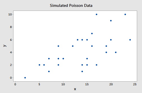
To illustrate consider this example (Poisson Simulated data), which consists of a simulated data set of size n = 30 such that the response (Y) follows a Poisson distribution with the rate $\lambda=\exp\{0.50+0.07X\}$. A plot of the response versus the predictor is given below.
The following gives the analysis of the Poisson regression data in Minitab:
- Select Stat > Regression > Poisson Regression > Fit Poisson Model.
- Select "y" for the Response.
- Select "x" as a Continuous predictor.
- Click Results and change "Display of results" to "Expanded tables."
This results in the following output:
Coefficients
| Term | Coef | SE Coef | 95% CI | Z-Value | P-Value | VIF |
|---|---|---|---|---|---|---|
| Constant | 0.308 | 0.289 | (-0.259, 0.875) | 1.06 | 0.287 | |
| x | 0.0764 | 0.0173 | (0.0424, 0.1103) | 4.41 | 0.000 | 1.00 |
Regression Equation
y = exp(Y')
Y' = 0.308 + 0.0764 x
As you can see, the Wald test p-value for x of 0.000 indicates that the predictor is highly significant.
Deviance Test
Changes in the deviance can be used to test the null hypothesis that any subset of the \(\beta\)'s is equal to 0. The deviance, \(D(\hat{\beta})\), is \(-2\) times the difference between the log-likelihood evaluated at the maximum likelihood estimate and the log-likelihood for a "saturated model" (a theoretical model with a separate parameter for each observation and thus a perfect fit). Suppose we test that r < p of the $\beta$'s are equal to 0. Then the deviance test statistic is given by:
\(\begin{equation*}
G^2=D(\hat{\beta}^{(0)})-D(\hat{\beta}),
\end{equation*}\)
where \(D(\hat{\beta})\) is the deviance of the fitted (full) model and \(D(\hat{\beta}^{(0)})\) is the deviance of the model specified by the null hypothesis evaluated at the maximum likelihood estimate of that reduced model. This test statistic has a \(\chi^{2}\) distribution with \(p-r\) degrees of freedom. This test procedure is analogous to the general linear F test procedure for multiple linear regression.
To illustrate, the relevant Minitab output from the simulated example is:
Deviance Table
| Source | DF | Seq Dev | Contribution | Adj Dev | Adj Mean | Chi-Square | P-Value |
|---|---|---|---|---|---|---|---|
| Regression | 1 | 20.47 | 42.37% | 20.47 | 20.4677 | 20.47 | 0.000 |
| x | 1 | 20.47 | 42.37% | 20.47 | 20.4677 | 20.47 | 0.000 |
| Error | 28 | 27.84 | 57.63% | 27.84 | 0.9944 | ||
| Total | 29 | 48.31 | 100.00% |
Since there is only a single predictor for this example, this table simply provides information on the deviance test for x (p-value of 0.000), which matches the earlier Wald test result (p-value of 0.000). (Note that the Wald test and deviance test will not in general give identical results.) The Deviance Table includes the following:
- The null model in this case has no predictors, so the fitted values are simply the sample mean, \(4.233\). The deviance for the null model is \(D(\hat{\beta}^{(0)})=48.31\), which is shown in the "Total" row in the Deviance Table.
- The deviance for the fitted model is \(D(\hat{\beta})=27.84\), which is shown in the "Error" row in the Deviance Table.
- The deviance test statistic is therefore \(G^2=48.31-27.84=20.47\).
- The p-value comes from a $\chi^{2}$ distribution with \(2-1=1\) degrees of freedom.
Goodness-of-Fit
The overall performance of the fitted model can be measured by two different chi-square tests. There is the Pearson statistic
\(\begin{equation*}
X^2=\sum_{i=1}^{n}\dfrac{(y_{i}-\exp\{\textbf{X}_{i}\hat{\beta}\})^{2}}{\exp\{\textbf{X}_{i}\hat{\beta}\}}
\end{equation*}\)
and the deviance statistic
\(\begin{equation*}
D=2\sum_{i=1}^{n}\biggl(y_{i}\log\biggl(\dfrac{y_{i}}{\exp\{\textbf{X}_{i}\hat{\beta}\}}\biggr)-(y_{i}-\exp\{\textbf{X}_{i}\hat{\beta}\})\biggr).
\end{equation*}\)
Both of these statistics are approximately chi-square distributed with n - p degrees of freedom. When a test is rejected, there is a statistically significant lack of fit. Otherwise, there is no evidence of a lack of fit.
To illustrate, the relevant Minitab output from the simulated example is:
Goodness-of-Fit
| Test | DF | Estimate | Mean | Chi-Square | P-Value |
|---|---|---|---|---|---|
| Deviance | 28 | 27.84209 | 0.099436 | 27.84 | 0.473 |
| Pearson | 28 | 26.09324 | 0.93190 | 26.09 | 0.568 |
The high p-values indicate no evidence of a lack of fit.
Overdispersion means that the actual covariance matrix for the observed data exceeds that for the specified model for \(Y|\textbf{X}\). For a Poisson distribution, the mean and the variance are equal. In practice, the data rarely reflects this fact and we have overdispersion in the Poisson regression model if (as is often the case) the variance is greater than the mean. In addition to testing goodness-of-fit, the Pearson statistic can also be used as a test of overdispersion. Note that overdispersion can also be measured in the logistic regression models that were discussed earlier.
Pseudo \(R^{2}\)
The value of \(R^{2}\) used in linear regression also does not extend to Poisson regression. One commonly used measure is the pseudo \(R^{2}\), defined as
\(\begin{equation*}
R^{2}=\dfrac{\ell(\hat{\beta_{0}})-\ell(\hat{\beta})}{\ell(\hat{\beta_{0}})}=1-\dfrac{D(\hat{\beta})}{D(\hat{\beta_{0}})},
\end{equation*}\)
where \(\ell(\hat{\beta_{0}})\) is the log-likelihood of the model when only the intercept is included. The pseudo \(R^{2}\) goes from 0 to 1 with 1 being a perfect fit.
To illustrate, the relevant Minitab output from the simulated example is:
Model Summary
| Deviance R-Sq |
Deviance R-Sq(adj) |
AIC |
|---|---|---|
| 42.37% | 40.30% | 124.50 |
Recall from above that \(D(\hat{\beta})=27.84\) and \(D(\hat{\beta}^{(0)})=48.31\), so:
\(\begin{equation*}
R^{2}=1-\dfrac{27.84}{48.31}=0.4237.
\end{equation*}\)
Raw Residual
The raw residual is the difference between the actual response and the estimated value from the model. Remember that the variance is equal to the mean for a Poisson random variable. Therefore, we expect that the variances of the residuals are unequal. This can lead to difficulties in the interpretation of the raw residuals, yet it is still used. The formula for the raw residual is
\(\begin{equation*}
r_{i}=y_{i}-\exp\{\textbf{X}_{i}\beta\}.
\end{equation*}\)
Pearson Residual
The Pearson residual corrects for the unequal variance in the raw residuals by dividing by the standard deviation. The formula for the Pearson residuals is
\(\begin{equation*}
p_{i}=\dfrac{r_{i}}{\sqrt{\hat{\phi}\exp\{\textbf{X}_{i}\beta\}}},
\end{equation*}\)
where
\(\begin{equation*}
\hat{\phi}=\dfrac{1}{n-p}\sum_{i=1}^{n}\frac{(y_{i}-\exp\{\textbf{X}_{i}\hat{\beta}\})^{2}}{\exp\{\textbf{X}_{i}\hat{\beta}\}}.
\end{equation*}\)
\(\hat{\phi}\) is a dispersion parameter to help control overdispersion.
Deviance Residuals
Deviance residuals are also popular because the sum of squares of these residuals is the deviance statistic. The formula for the deviance residual is
\(\begin{equation*}
d_{i}=\texttt{sgn}(y_{i}-\exp\{\textbf{X}_{i}\hat{\beta}\})\sqrt{2\biggl\{y_{i}\log\biggl(\dfrac{y_{i}}{\exp\{\textbf{X}_{i}\hat{\beta}\}}\biggr)-(y_{i}-\exp\{\textbf{X}_{i}\hat{\beta}\})\biggr\}}.
\end{equation*}\)
The plots below show the Pearson residuals and deviance residuals versus the fitted values for the simulated example.
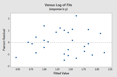
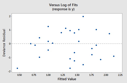
These plots appear to be good for a Poisson fit. Further diagnostic plots can also be produced and model selection techniques can be employed when faced with multiple predictors.
Hat Values
The hat matrix serves the same purpose as in the case of linear regression - to measure the influence of each observation on the overall fit of the model. The hat values, \(h_{i,i}\), are the diagonal entries of the Hat matrix
\(\begin{equation*}
H=\textbf{W}^{1/2}\textbf{X}(\textbf{X}\textbf{W}\textbf{X})^{-1}\textbf{X}\textbf{W}^{1/2},
\end{equation*}\)
where W is an \(n\times n\) diagonal matrix with the values of $\exp\{\textbf{X}_{i}\hat{\beta}\}$ on the diagonal. As before, a hat value (leverage) is large if \(h_{i,i}>2p/n\).
Studentized Residuals
Finally, we can also report Studentized versions of some of the earlier residuals. The Studentized Pearson residuals are given by
\(\begin{equation*}
sp_{i}=\dfrac{p_{i}}{\sqrt{1-h_{i,i}}}
\end{equation*}\)
and the Studentized deviance residuals are given by
\(\begin{equation*}
sd_{i}=\dfrac{d_{i}}{\sqrt{1-h_{i, i}}}.
\end{equation*}\)
To illustrate, the relevant Minitab output from the simulated example is:
Fits and Diagnostics for Unusual Observations
| Obs | y | Fit | SE Fit | 95% CI | Resid | Std Resid | Del Resid | HI | Cook's D |
|---|---|---|---|---|---|---|---|---|---|
| 8 | 10.000 | 4.983 | 0.452 | (4.171, 5.952) | 1.974 | 2.02 | 2.03 | 0.040969 | 0.11 |
| 21 | 6.000 | 8.503 | 1.408 | (6.147, 11.763) | -0.907 | -1.04 | -1.02 | 0.233132 | 0.15 |
Fits and Diagnostics for Unusual Observation
| Obs | DFITS | ||
|---|---|---|---|
| 8 | 0.474408 | R | |
| 21 | -0.540485 | X |
R large residual
X Unusual X
The default residuals in this output (set under Minitab's Regression Options) are deviance residuals, so observation 8 has a deviance residual of 1.974 and studentized deviance residual of 2.02, while observation 21 has leverage (h) of 0.233132.
T.3.2 - Polytomous Regression
T.3.2 - Polytomous RegressionIn binary logistic regression, we only had two possible outcomes. For polytomous logistic regression, we will consider the possibility of having k > 2 possible outcomes. (Note: The word polychotomous is sometimes used, but note that this is not actually a word!)
Nominal Logistic Regression
The multiple nominal logistic regression model (sometimes called the multinomial logistic regression model) is given by the following:
\(\begin{equation}\label{nommod}
\pi_{j}=\left\{
\begin{array}{ll}
\dfrac{\exp(\textbf{X}\beta_{j})}{1+\sum_{j=2}^{k}\exp(\textbf{X}\beta_{j})} & \hbox{j=2,...,k} \\
\\
\dfrac{1}{1+\sum_{j=2}^{k}\exp(\textbf{X}\beta_{j})}
& \hbox{j=1} \end{array} \right.
\end{equation}\)
where again \(\pi_{j}\) denotes a probability and not the irrational number. Notice that k - 1 of the groups has its own set of \(\beta\) values. Furthermore, since \(\sum_{j=1}^{k}\pi_{j}=1\), we set the \(\beta\) values for group 1 to be 0 (this is what we call the reference group). Notice that when k = 2, we are back to binary logistic regression.
\(\pi_{j}\) is the probability that an observation is in one of the k categories. The likelihood for the nominal logistic regression model is given by:
\(\begin{align*}
L(\beta;\textbf{y},\textbf{X})&=\prod_{i=1}^{n}\prod_{j=1}^{k}\pi_{i,j}^{y_{i,j}}(1-\pi_{i,j})^{1-y_{i,j}},
\end{align*}\)
where the subscript \((i,j)\) means the \(i^{\textrm{th}}\) observation belongs to the \(j^{\textrm{th}}\) group. This yields the log-likelihood:
\(\begin{equation*}
\ell(\beta)=\sum_{i=1}^{n}\sum_{j=1}^{k}y_{i,j}\pi_{i,j}.
\end{equation*}\)
Maximizing the likelihood (or log-likelihood) has no closed-form solution, so a technique like iteratively reweighted least squares is used to find an estimate of the regression coefficients, \(\hat{\beta}\).
An odds ratio (\(\theta\)) of 1 serves as the baseline for comparison. If \(\theta=1\), then there is no association between the response and predictor. If \(\theta>1 \), then the odds of success are higher for the indicated level of the factor (or for higher levels of a continuous predictor). If \(\theta<1 \), then the odds of success are less for the indicated level of the factor (or for higher levels of a continuous predictor). Values farther from 1 represent stronger degrees of association. For nominal logistic regression, the odds of success (at two different levels of the predictors, say \(\textbf{X}_{(1)}\) and \(\textbf{X}_{(2)}\)) are:
\(\begin{equation*}
\theta=\dfrac{(\pi_{j}/\pi_{1})|_{\textbf{X}=\textbf{X}_{(1)}}}{(\pi_{j}/\pi_{1})|_{\textbf{X}=\textbf{X}_{(2)}}}.
\end{equation*}\)
Many of the procedures discussed in binary logistic regression can be extended to nominal logistic regression with the appropriate modifications.
Ordinal Logistic Regression
For ordinal logistic regression, we again consider k possible outcomes as in nominal logistic regression, except that the order matters. The multiple ordinal logistic regression model is the following:
\(\begin{equation}\label{ordmod}
\sum_{j=1}^{k^{*}}\pi_{j}=\dfrac{\exp(\beta_{0,k^{*}}+\textbf{X}\beta)}{1+\exp(\beta_{0,k^{*}}+\textbf{X}\beta)}
\end{equation}\)
such that \(k^{*}\leq k\), \(\pi_{1}\leq\pi_{2},\leq \ldots,\leq\pi_{k}\), and again \(\pi_{j}\) denotes a probability. Notice that this model is a cumulative sum of probabilities which involves just changing the intercept of the linear regression portion (so \(\beta\) is now (p - 1)-dimensional and X is \(n\times(p-1)\) such that first column of this matrix is not a column of 1's). Also, it still holds that \(\sum_{j=1}^{k}\pi_{j}=1\).
\(\pi_{j}\) is still the probability that an observation is in one of the k categories, but we are constrained by the model written in the equation above. The likelihood for the ordinal logistic regression model is given by:
\(\begin{align*}
L(\beta;\textbf{y},\textbf{X})&=\prod_{i=1}^{n}\prod_{j=1}^{k}\pi_{i,j}^{y_{i,j}}(1-\pi_{i,j})^{1-y_{i,j}},
\end{align*}\)
where the subscript (i, j) means the \(i^{\textrm{th}}\) observation belongs to the \(j^{\textrm{th}}\) group. This yields the log-likelihood:
\(\begin{equation*}
\ell(\beta)=\sum_{i=1}^{n}\sum_{j=1}^{k}y_{i,j}\pi_{i,j}.
\end{equation*}\)
Notice that this is identical to the nominal logistic regression likelihood. Thus, maximization again has no closed-form solution, so we defer to a procedure like iteratively reweighted least squares.
For ordinal logistic regression, a proportional odds model is used to determine the odds ratio. Again, an odds ratio (\(\theta\)) of 1 serves as the baseline for comparison between the two predictor levels, say \(\textbf{X}_{(1)}\) and \(\textbf{X}_{(2)}\). Only one parameter and one odds ratio is calculated for each predictor. Suppose we are interested in calculating the odds of \(\textbf{X}_{(1)}\) to \(\textbf{X}_{(2)}\). If \(\theta=1\), then there is no association between the response and these two predictors. If \(\theta>1\), then the odds of success are higher for the predictor \(\textbf{X}_{(1)}\). If \(\theta<1\), then the odds of success are less for the predictor \(\textbf{X}_{(1)}\). Values farther from 1 represent stronger degrees of association. For ordinal logistic regression, the odds ratio utilizes cumulative probabilities and their complements and is given by:
\(\begin{equation*}
\theta=\dfrac{\sum_{j=1}^{k^{*}}\pi_{j}|_{\textbf{X}=\textbf{X}_{(1)}}/(1-\sum_{j=1}^{k^{*}}\pi_{j})|_{\textbf{X}=\textbf{X}_{(1)}}}{\sum_{j=1}^{k^{*}}\pi_{j}|_{\textbf{X}=\textbf{X}_{(2)}}/(1\sum_{j=1}^{k^{*}}\pi_{j})|_{\textbf{X}=\textbf{X}_{(2)}}}.
\end{equation*}\)
T.3.3 - Generalized Linear Models
T.3.3 - Generalized Linear ModelsAll of the regression models we have considered (including multiple linear, logistic, and Poisson) belong to a family of models called generalized linear models. (In fact, a more "generalized" framework for regression models is called general regression models, which includes any parametric regression model.) Generalized linear models provide a generalization of ordinary least squares regression that relates the random term (the response Y) to the systematic term (the linear predictor \(\textbf{X}\beta\)) via a link function (denoted by \(g(\cdot)\)). Specifically, we have the relation
\(\begin{equation*}
\mbox{E}(Y)=\mu=g^{-1}(\textbf{X}\beta),
\end{equation*}\)
so \(g(\mu)=\textbf{X}\beta\). Some common link functions are:
- Identity Link
-
The identity link:
\(\begin{equation*}
g(\mu)=\mu=\textbf{X}\beta,
\end{equation*}\)which is used in traditional linear regression.
- Logit Link
-
The logit link:
\(\begin{align*}
&g(\mu)=\log\biggl(\frac{\mu}{1-\mu}\biggr)=\textbf{X}\beta\\
&\Rightarrow\mu=\frac{e^{\textbf{X}\beta}}{1+e^{\textbf{X}\beta}},
\end{align*}\)which is used in logistic regression.
- Log Link
-
The log link:
\(\begin{align*}
&g(\mu)=\log(\mu)=\textbf{X}\beta\\
&\Rightarrow\mu=e^{\textbf{X}\beta},
\end{align*}\)which is used in Poisson regression.
- Probit Link
-
The probit link:
\(\begin{align*}
&g(\mu)=\Phi^{-1}(\mu)=\textbf{X}\beta\\
&\Rightarrow\mu=\Phi(\textbf{X}\beta),
\end{align*}\)where \(\Phi(\cdot)\) is the cumulative distribution function of the standard normal distribution. This link function is also sometimes called the normit link. This also can be used in logistic regression.
- Complementary Log-Log Link
-
The complementary log-log link:
\(\begin{align*}
&g(\mu)=\log(-\log(1-\mu))=\textbf{X}\beta\\
&\Rightarrow\mu=1-\exp\{-e^{\textbf{X}\beta}\},
\end{align*}\)which can also be used in logistic regression. This link function is also sometimes called the gompit link.
- Power Link
-
The power link:
\(\begin{align*}
&g(\mu)=\mu^{\lambda}=\textbf{X}\beta\\
&\Rightarrow\mu=(\textbf{X}\beta)^{1/\lambda},
\end{align*}\)where \(\lambda\neq 0\). This is used in other regressions which we do not explore (such as gamma regression and inverse Gaussian regression).
Also, the variance is typically a function of the mean and is often written as
\(\begin{equation*}
\mbox{Var}(Y)=V(\mu)=V(g^{-1}(\textbf{X}\beta)).
\end{equation*}\)
The random variable Y is assumed to belong to an exponential family distribution where the density can be expressed in the form
\(\begin{equation*}
q(y;\theta,\phi)=\exp\biggl\{\dfrac{y\theta-b(\theta)}{a(\phi)}+c(y,\phi)\biggr\},
\end{equation*}\)
where \(a(\cdot)\), \(b(\cdot)\), and \(c(\cdot)\) are specified functions, \(\theta\) is a parameter related to the mean of the distribution, and \(\phi\) is called the dispersion parameter. Many probability distributions belong to the exponential family. For example, the normal distribution is used for traditional linear regression, the binomial distribution is used for logistic regression, and the Poisson distribution is used for Poisson regression. Other exponential family distributions lead to gamma regression, inverse Gaussian (normal) regression, and negative binomial regression, just to name a few.
The unknown parameters, \(\beta\), are typically estimated with maximum likelihood techniques (in particular, using iteratively reweighted least squares), Bayesian methods, or quasi-likelihood methods. The quasi-likelihood is a function that possesses similar properties to the log-likelihood function and is most often used with count or binary data. Specifically, for a realization y of the random variable Y, it is defined as
\(\begin{equation*}
Q(\mu;y)=\int_{y}^{\mu}\dfrac{y-t}{\sigma^{2}V(t)}dt,
\end{equation*}\)
where \(\sigma^{2}\) is a scale parameter. There are also tests using likelihood ratio statistics for model development to determine if any predictors may be dropped from the model.
T.3.4 - Nonlinear Regression
T.3.4 - Nonlinear RegressionAll of the models we have discussed thus far have been linear in the parameters (i.e., linear in the beta's). For example, polynomial regression was used to model curvature in our data by using higher-ordered values of the predictors. However, the final regression model was just a linear combination of higher-ordered predictors.
Now we are interested in studying the nonlinear regression model:
\(\begin{equation*}
Y=f(\textbf{X},\beta)+\epsilon,
\end{equation*}\)
where X is a vector of p predictors, \(\beta\) is a vector of k parameters, \(f(\cdot)\) is some known regression function, and \(\epsilon\) is an error term whose distribution may or may not be normal. Notice that we no longer necessarily have the dimension of the parameter vector simply one greater than the number of predictors. Some examples of nonlinear regression models are:
\(\begin{align*}
y_{i}&=\frac{e^{\beta_{0}+\beta_{1}x_{i}}}{1+e^{\beta_{0}+\beta_{1}x_{i}}}+\epsilon_{i} \\
y_{i}&=\frac{\beta_{0}+\beta_{1}x_{i}}{1+\beta_{2}e^{\beta_{3}x_{i}}}+\epsilon_{i} \\
y_{i}&=\beta_{0}+(0.4-\beta_{0})e^{-\beta_{1}(x_{i}-5)}+\epsilon_{i}.
\end{align*}\)
However, there are some nonlinear models which are actually called intrinsically linear because they can be made linear in the parameters by a simple transformation. For example:
\(\begin{equation*}
Y=\frac{\beta_{0}X}{\beta_{1}+X}
\end{equation*}\)
can be rewritten as
\(\begin{align*}
\frac{1}{Y}&=\frac{1}{\beta_{0}}+\frac{\beta_{1}}{\beta_{0}}\frac{1}{X}\\
&=\theta_{0}+\theta_{1}\frac{1}{X},
\end{align*}\)
which is linear in the transformed parameters \(\theta_{0}\) and \(\theta_{1}\). In such cases, transforming a model to its linear form often provides better inference procedures and confidence intervals, but one must be cognizant of the effects that the transformation has on the distribution of the errors.
Nonlinear Least Squares
Returning to cases in which it is not possible to transform the model to a linear form, consider the setting
\(\begin{equation*}
Y_{i}=f(\textbf{X}_{i},\beta)+\epsilon_{i},
\end{equation*}\)
where the \(\epsilon_{i}\) are iid normal with mean 0 and constant variance \(\sigma^{2}\). For this setting, we can rely on some of the least squares theories we have developed over the course. For other nonnormal error terms, different techniques need to be employed.
First, let
\(\begin{equation*}
Q=\sum_{i=1}^{n}(y_{i}-f(\textbf{X}_{i},\beta))^{2}.
\end{equation*}\)
In order to find
\(\begin{equation*}
\hat{\beta}=\arg\min_{\beta}Q,
\end{equation*}\)
we first find each of the partial derivatives of Q with respect to \(\beta_{j}\). Then, we set each of the partial derivatives equal to 0 and the parameters \(\beta_{k}\) are each replaced by \(\hat{\beta}_{k}\). The functions to be solved are nonlinear in the parameter estimates \(\hat{\beta}_{k}\) and are often difficult to solve, even in the simplest cases. Hence, iterative numerical methods are often employed. Even more difficulty arises in that multiple solutions may be possible!
Algorithms for nonlinear least squares estimation include:
- Newton's method
- is a classical method based on a gradient approach but which can be computationally challenging and heavily dependent on good starting values.
- Gauss-Newton algorithm
- is a modification of Newton's method that gives a good approximation of the solution that Newton's method should have arrived at but which is not guaranteed to converge.
- Levenberg-Marquardt method
- can take care of computational difficulties arising from the other methods but can require a tedious search for the optimal value of a tuning parameter.
T.3.5 - Exponential Regression Example
T.3.5 - Exponential Regression ExampleOne simple nonlinear model is the exponential regression model
\(\begin{equation*}
y_{i}=\beta_{0}+\beta_{1}\exp(\beta_{2}x_{i,1}+\ldots+\beta_{p+1}x_{i,1})+\epsilon_{i},
\end{equation*}\)
where the \(\epsilon_{i}\) are iid normal with mean 0 and constant variance \(\sigma^{2}\). Notice that if \(\beta_{0}=0\), then the above is intrinsically linear by taking the natural logarithm of both sides.
Exponential regression is probably one of the simplest nonlinear regression models. An example where an exponential regression is often utilized is when relating the concentration of a substance (the response) to elapsed time (the predictor).
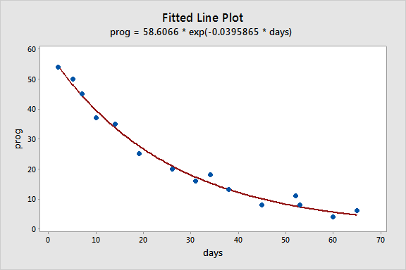
To illustrate, consider the example of long-term recovery after discharge from the hospital from page 514 of Applied Linear Regression Models (4th ed) by Kutner, Nachtsheim, and Neter. The response variable, Y, is the prognostic index for long-term recovery, and the predictor variable, X, is the number of days of hospitalization. The proposed model is the two-parameter exponential model:
\(\begin{equation*}
Y_{i}=\theta_{0}\exp(\theta_{1}X_i)+\epsilon_{i},
\end{equation*}\)
where the \(\epsilon_i\) are independent normal with constant variance.
We'll use Minitab's nonlinear regression routine to apply the Gauss-Newton algorithm to estimate \(\theta_0\) and \(\theta_1\). Before we do this, however, we have to find initial values for \(\theta_0\) and \(\theta_1\). One way to do this is to note that we can linearize the response function by taking the natural logarithm:
\(\begin{equation*}
\log(\theta_{0}\exp(\theta_{1}X_i)) = \log(\theta_{0}) + \theta_{1}X_i.
\end{equation*}\)
Thus we can fit a simple linear regression model with the response, \(\log(Y)\), and predictor, \(X\), and the intercept (\(4.0372\)) give us an estimate of \(\log(\theta_{0})\) while the slope (\(-0.03797\)) gives us an estimate of \(\theta_{1}\). (We then calculate \(\exp(4.0372)=56.7\) to estimate \(\theta_0\).)
Minitab: Nonlinear Regression Model
Now we can fit the nonlinear regression model:
- Select Stat > Regression > Nonlinear Regression, select prog for the response, and click "Use Catalog" under "Expectation Function."
- Select the "Exponential" function with 1 predictor and 2 parameters in the Catalog dialog box and click OK to go to the "Choose Predictors" dialog.
- Select days to be the "Actual predictor" and click OK to go back to the Catalog dialog box, where you should see "Theta1 * exp( Theta2 * days )" in the "Expectation Function" box.
- Click "Parameters" and type "56.7" next to "Theta1" and "-0.038" next to "Theta2" and click OK to go back to the Nonlinear Regression dialog box.
- Click "Options" to confirm that Minitab will use the Gauss-Newton algorithm (the other choice is Levenberg-Marquardt) and click OK to go back to the Nonlinear Regression dialog box.
- Click "Graphs" to confirm that Minitab will produce a plot of the fitted curve with data and click OK to go back to the Nonlinear Regression dialog box.
- Click OK to obtain the following output:
Nonlinear Regression: Prog = Theta1 * exp(Theta2 * days)
| Algorithm | Gauss-Newton |
|---|---|
| Max iterations | 200 |
| Tolerance | 0.00001 |
| Parameter | Value |
|---|---|
| Theta1 | 56.7 |
| Theta2 | -0.038 |
Equation
prog = 58.6066 * exp(-0.0395865 * days)
| Parameter | Estimate | SE Estimate |
|---|---|---|
| Theta1 | 58.6066 | 1.47216 |
| Theta2 | 0.0396 | 0.00171 |
prog = Theta1 * exp(Theta2 * days)
| Iterations | 5 |
|---|---|
| Final SSE | 49.4593 |
| DFE | 13 |
| MSE | 3.80456 |
| S | 1.95053 |
T.3.6 - Population Growth Example
T.3.6 - Population Growth ExampleCensus Data

A simple model for population growth towards an asymptote is the logistic model
\(\begin{equation*}
y_{i}=\dfrac{\beta_{1}}{1+\exp(\beta_{2}+\beta_{3}x_{i})}+\epsilon_{i},
\end{equation*}\)
where \(y_{i}\) is the population size at time \(x_{i}\), \(\beta_{1}\) is the asymptote towards which the population grows, \(\beta_{2}\) reflects the size of the population at time x = 0 (relative to its asymptotic size), and \(\beta_{3}\) controls the growth rate of the population.
We fit this model to Census population data (US Census data) for the United States (in millions) ranging from 1790 through 1990 (see below).
| year | population |
|---|---|
| 1790 | 3.929 |
| 1800 | 5.308 |
| 1810 | 7.240 |
| 1820 | 9.638 |
| 1830 | 12.866 |
| 1840 | 17.069 |
| 1850 | 23.192 |
| 1860 | 31.443 |
| 1870 | 39.818 |
| 1880 | 50.156 |
| 1890 | 62.948 |
| 1900 | 75.995 |
| 1910 | 91.972 |
| 1920 | 105.711 |
| 1930 | 122.775 |
| 1940 | 131.669 |
| 1950 | 150.697 |
| 1960 | 179.323 |
| 1970 | 203.302 |
| 1980 | 226.542 |
| 1990 | 248.710 |
The data are graphed (see below) and the line represents the fit of the logistic population growth model.
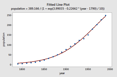
To fit the logistic model to the U. S. Census data, we need starting values for the parameters. It is often important in nonlinear least squares estimation to choose reasonable starting values, which generally requires some insight into the structure of the model. We know that \(\beta_{1}\) represents asymptotic population. The data in the plot above show that in 1990 the U. S. population stood at about 250 million and did not appear to be close to an asymptote; so as not to extrapolate too far beyond the data, let us set the starting value of \(\beta_{1}\) to 350. It is convenient to scale time so that \(x_{1}=0\) in 1790, and so that the unit of time is 10 years.
Then substituting \(\beta_{1}=350\) and \(x=0\) into the model, using the value \(y_{1}=3.929\) from the data, and assuming that the error is 0, we have
\(\begin{equation*}
3.929=\dfrac{350}{1+\exp(\beta_{2}+\beta_{3}(0))}.
\end{equation*}\)
Solving for \(\beta_{2}\) gives us a plausible start value for this parameter:
\(\begin{align*}
\exp(\beta_{2})&=\dfrac{350}{3.929}-1\\
\beta_{2}&=\log\biggl(\frac{350}{3.929}-1\biggr)\approx 4.5.
\end{align*}\)
Finally, returning to the data, at time x = 1 (i.e., at the second Census performed in 1800), the population was \(y_{2}=5.308\). Using this value, along with the previously determined start values for \(\beta_{1}\) and \(\beta_{2}\), and again setting the error to 0, we have
\(\begin{equation*}
5.308=\dfrac{350}{1+\exp(4.5+\beta_{3}(1))}.
\end{equation*}\)
Solving for \(\beta_{3}\) we get
\(\begin{align*}
\exp(4.5+\beta_{3})&=\frac{350}{5.308}-1\\
\beta_{3}&=\log\biggl(\dfrac{350}{5.308}-1\biggr)-4.5\approx -0.3.
\end{align*}\)
So now we have starting values for the nonlinear least squares algorithm that we use. Below is the output from fitting the model in Minitab using Gauss-Netwon:
- Select Stat > Regression > Nonlinear Regression
- Select "population" for the Response
- Type the following into the "Edit directly" box under Expectation Function: beta1/(1+exp(beta2+beta3*(year-1790)/10))
- Click Parameters and type in the values specified above (350, 4.5, and –0.3)
As you can see, the starting values resulted in convergence with values not too far from our guess.
Equation
population = 389.166/(1+exp(3.99035 - 0.22662 * (year - 1790) / 10))
Parameter Estimates
| Paraemeter | Estimate | SE Estimate |
|---|---|---|
| beta1 | 389.166 | 30.8120 |
| beta2 | 3.990 | 0.0703 |
| beta3 | -0.227 | 0.0109 |
population = beta1/(1 + exp(beta2 + beta3 * (year - 1790) / 10))
Lack of Fit
There are no replicates.
Minitab cannot do the lack of fit test based on pure errror.
Summary
| Iterations | 8 |
|---|---|
|
Final SSE |
356.400 |
| DFE | 18 |
| MSE | 19.8000 |
| S | 4.44972 |
Here is a plot of the residuals versus the year.
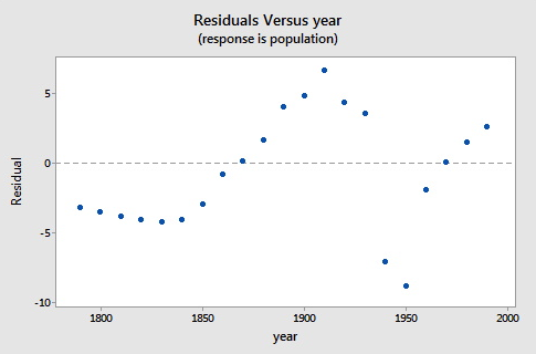
As you can see, the logistic functional form that we chose did catch the gross characteristics of this data, but some of the nuances appear to not be as well characterized. Since there are indications of some cyclical behavior, a model incorporating correlated errors or, perhaps, trigonometric functions could be investigated.
Software Help: Poisson & Nonlinear Regression
Software Help: Poisson & Nonlinear Regression
The next two pages cover the Minitab and R commands for the procedures in this lesson.
Below is a file that contains the data set used in this help section:
Minitab Help: Poisson & Nonlinear Regression
Minitab Help: Poisson & Nonlinear RegressionMinitab®
Hospital recovery (exponential regression)
- Select Calc > Calculator to create a log(prog) variable.
- Obtain starting values for nonlinear model parameters from fitting a simple linear regression model of log(prog) vs days.
- Select Stat > Regression > Nonlinear Regression to fit a nonlinear regression model to data using these starting values. Put prog in the "Response" box and type "Theta1 * exp(Theta2 * days)" into the box labeled "Edit directly." Before clicking OK, click "Parameters" and enter 56.7 as the starting value for Theta1 and -0.038 as the starting value for Theta2.
- A scatterplot of prog vs days with a fitted line based on the nonlinear regression model is produced by default.
U.S. Census population (population growth nonlinear regression)
- Obtain starting values for nonlinear model parameters from observing features of a scatterplot of population vs year.
- Select Stat > Regression > Nonlinear Regression to fit a nonlinear regression model to data using these starting values. Put population in the "Response" box and type "beta1 / (1 + exp(beta2 + beta3 * (year - 1790) / 10))" into the box labeled "Edit directly." Before clicking OK, click "Parameters" and enter 56.7 as the starting value for Theta1 and -0.038 as the starting value for Theta2.
- A scatterplot of population vs year with a fitted line based on the nonlinear regression model is produced by default.
- Before clicking "OK" in the Regression Dialog, click "Graphs" and put the year in the "Residuals versus the variables" box.
Poisson example (Poisson regression)
- Select Graph > Scatterplot to create a scatterplot of the data.
- Select Stat > Regression > Poisson Regression > Fit Poisson Model, put y in the "Response" box, and put x in the "Continuous predictors" box. Before clicking "OK," click "Results" and select "Expanded tables" for "Display of results."
- Before clicking "OK" in the Regression Dialog, click "Graphs" and select "Residuals versus Fits" to create residual plots using deviance residuals. To change to Pearson residuals, click "Options" in the Regression Dialog and select "Pearson" for "Residuals for diagnostics."
R Help: Poisson & Nonlinear Regression
R Help: Poisson & Nonlinear RegressionHospital recovery (exponential regression)
- Load the recovery data.
- Create log(prog) variable.
- Obtain starting values for nonlinear model parameters from fitting a simple linear regression model of log(prog) vs days.
- Fit nonlinear regression model to data using these starting values.
- Create a scatterplot of prog vs days and add a fitted line based on the nonlinear regression model.
recovery <- read.table("~/path-to-data/recovery.txt", header=T)
attach(recovery)
logprog <- log(prog)
summary(lm(logprog ~ days))
#              Estimate Std. Error t value Pr(>|t|)
# (Intercept)  4.037159   0.084103   48.00 5.08e-16 ***
# days        -0.037974   0.002284  -16.62 3.86e-10 ***
exp(4.037159) # 56.66513
model.1 <- nls(prog ~ theta1 * exp(theta2 * days),
start=list(theta1=56.7, theta2=-0.038))
summary(model.1)
#         Estimate Std. Error t value Pr(>|t|)
# theta1 58.606532   1.472159   39.81 5.70e-15 ***
# theta2 -0.039586   0.001711  -23.13 6.01e-12 ***
# ---
# Residual standard error: 1.951 on 13 degrees of freedom
plot(x=days, y=prog,
panel.last = lines(sort(days), fitted(model.1)[order(days)]))
detach(recovery)
U.S. Census population (population growth nonlinear regression)
- Load the census data.
- Obtain starting values for nonlinear model parameters from observing features of a scatterplot of population vs year.
- Fit nonlinear regression model to data using these starting values.
- Create a scatterplot of population vs year and add a fitted line based on the nonlinear regression model.
- Create a residual plot.
census <- read.table("~/path-to-data/us_census.txt", header=T)
attach(census)
plot(x=year, y=population)
log(350/3.929-1) # 4.478259
log(350/5.308-1) - log(350/3.929-1) # -0.3048229
model.1 <- nls(population ~ beta1 / (1 + exp(beta2 + beta3 * (year - 1790) / 10)),
start=list(beta1=350, beta2=4.5, beta3=-0.3))
summary(model.1)
#        Estimate Std. Error t value Pr(>|t|)
# beta1 389.16551   30.81196   12.63  2.2e-10 ***
# beta2   3.99035    0.07032   56.74  < 2e-16 ***
# beta3  -0.22662    0.01086  -20.87  4.6e-14 ***
# ---
# Residual standard error: 4.45 on 18 degrees of freedom
plot(x=year, y=population,
panel.last = lines(sort(year), fitted(model.1)[order(year)]))
plot(x=year, y=residuals(model.1),
panel.last = abline(h=0, lty=2))
detach(census)
Poisson example (Poisson regression)
- Load the poisson data.
- Create a scatterplot of the data.
- Fit a Poisson regression model of y vs x.
- Calculate 95% confidence intervals for the regression parameters based on asymptotic normality and based on profiling the least-squares estimation surface.
- Create a scatterplot of y vs x and add a fitted line based on the Poisson regression model.
- Conduct a likelihood ratio (or deviance) test for x.
- Calculate the sum of squared deviance residuals and the sum of squared Pearson residuals and calculate p-values based on chi-squared goodness-of-fit tests.
- Calculate pseudo \(R^2\) for Poisson regression.
- Create residual plots using Pearson and deviance residuals.
- Calculate hat values (leverages) and studentized residuals.
poisson <- read.table("~/path-to-data/poisson_simulated.txt", header=T)
attach(poisson)
plot(x=x, y=y)
model.1 <- glm(y ~ x, family="poisson")
summary(model.1)
#             Estimate Std. Error z value Pr(>|z|)
# (Intercept)  0.30787    0.28943   1.064    0.287
# x            0.07636    0.01730   4.413 1.02e-05 ***
# ---
# Signif. codes:  0 ‘***’ 0.001 ‘**’ 0.01 ‘*’ 0.05 ‘.’ 0.1 ‘ ’ 1
#
# (Dispersion parameter for poisson family taken to be 1)
#
# Null deviance: 48.310  on 29  degrees of freedom
# Residual deviance: 27.842  on 28  degrees of freedom
# AIC: 124.5
confint.default(model.1) # based on asymptotic normality
confint(model.1) # based on profiling the least-squares estimation surface
plot(x=x, y=y,
panel.last = lines(sort(x), fitted(model.1)[order(x)]))
anova(model.1, test="Chisq")
#      Df Deviance Resid. Df Resid. Dev  Pr(>Chi)
# NULL                    29     48.310
# x     1   20.468        28     27.842 6.065e-06 ***
sum(residuals(model.1, type="deviance")^2) # 27.84209
model.1$deviance # 27.84209
pchisq(model.1$deviance, 28, lower.tail=F) # p-value = 0.4728389
sum(residuals(model.1, type="pearson")^2) # 26.09324
pchisq(sum(residuals(model.1, type="pearson")^2), 28, lower.tail=F) # p-value = 0.5679192
1-model.1$deviance/model.1$null.deviance # Pseudo R-squared = 0.423676
plot(fitted(model.1), residuals(model.1, type="pearson"))
plot(fitted(model.1), residuals(model.1, type="deviance"))
summary(influence.measures(model.1))
#    dfb.1_ dfb.x dffit cov.r   cook.d hat
# 10 -0.22   0.30  0.37  1.25_*  0.08   0.18
# 21  0.37  -0.48 -0.57  1.30_*  0.15   0.23_*
residuals(model.1)[8] # 1.974329
rstudent(model.1)[8] # 2.028255
detach(poisson)