13.2 - Logistic Regression
13.2 - Logistic RegressionLogistic regression models a relationship between predictor variables and a categorical response variable. For example, we could use logistic regression to model the relationship between various measurements of a manufactured specimen (such as dimensions and chemical composition) to predict if a crack greater than 10 mils will occur (a binary variable: either yes or no). Logistic regression helps us estimate the probability of falling into a certain level of the categorical response given a set of predictors. We can choose from three types of logistic regression, depending on the nature of the categorical response variable:
- Binary Logistic Regression
- Used when the response is binary (i.e., it has two possible outcomes). The cracking example given above would utilize binary logistic regression. Other examples of binary responses could include passing or failing a test, responding yes or no on a survey, and having high or low blood pressure.
- Nominal Logistic Regression
- Used when there are three or more categories with no natural ordering to the levels. Examples of nominal responses could include departments at a business (e.g., marketing, sales, HR), type of search engine used (e.g., Google, Yahoo!, MSN), and color (black, red, blue, orange).
- Ordinal Logistic Regression
- Used when there are three or more categories with a natural ordering to the levels, but the ranking of the levels does not necessarily mean the intervals between them are equal. Examples of ordinal responses could be how students rate the effectiveness of a college course on a scale of 1-5, levels of flavors for hot wings, and medical condition (e.g., good, stable, serious, critical).
Particular issues with modeling a categorical response variable include nonnormal error terms, nonconstant error variance, and constraints on the response function (i.e., the response is bounded between 0 and 1). We will investigate ways of dealing with these in the binary logistic regression setting here. There is some discussion of the nominal and ordinal logistic regression settings in Section 15.2.
The multiple binary logistic regression model is the following:
\(\begin{align}\label{logmod}
\pi&=\dfrac{\exp(\beta_{0}+\beta_{1}X_{1}+\ldots+\beta_{p-1}X_{p-1})}{1+\exp(\beta_{0}+\beta_{1}X_{1}+\ldots+\beta_{p-1}X_{p-1})}\notag \\
&
=\dfrac{\exp(\textbf{X}\beta)}{1+\exp(\textbf{X}\beta)}\\
&
=\dfrac{1}{1+\exp(-\textbf{X}\beta)}
\end{align}\)
where here \(\pi\) denotes a probability and not the irrational number 3.14...
- \(\pi\) is the probability that an observation is in a specified category of the binary Y variable, generally called the "success probability."
- Notice that the model describes the probability of an event happening as a function of X variables. For instance, it might provide estimates of the probability that an older person has heart disease.
- With the logistic model, estimates of \(\pi\) from equations like the one above will always be between 0 and 1. The reasons are:
- The numerator \(\exp(\beta_{0}+\beta_{1}X_{1}+\ldots+\beta_{p-1}X_{p-1})\) must be positive because it is a power of a positive value (e).
- The denominator of the model is (1 + numerator), so the answer will always be less than 1.
- With one X variable, the theoretical model for \(\pi\) has an elongated "S" shape (or sigmoidal shape) with asymptotes at 0 and 1, although in sample estimates we may not see this "S" shape if the range of the X variable is limited.
For a sample of size n, the likelihood for a binary logistic regression is given by:
\(\begin{align*}
L(\beta;\textbf{y},\textbf{X})&=\prod_{i=1}^{n}\pi_{i}^{y_{i}}(1-\pi_{i})^{1-y_{i}}\\
&
=\prod_{i=1}^{n}\biggl(\dfrac{\exp(\textbf{X}_{i}\beta)}{1+\exp(\textbf{X}_{i}\beta)}\biggr)^{y_{i}}\biggl(\dfrac{1}{1+\exp(\textbf{X}_{i}\beta)}\biggr)^{1-y_{i}}.
\end{align*}\)
This yields the log-likelihood:
\(\begin{align*}
\ell(\beta)&=\sum_{i=1}^{n}(y_{i}\log(\pi_{i})+(1-y_{i})\log(1-\pi_{i}))\\
&
=\sum_{i=1}^{n}(y_{i}\textbf{X}_{i}\beta-\log(1+\exp(\textbf{X}_{i}\beta))).
\end{align*}\)
Maximizing the likelihood (or log-likelihood) has no closed-form solution, so a technique like iteratively reweighted least squares is used to find an estimate of the regression coefficients, \(\hat{\beta}\).
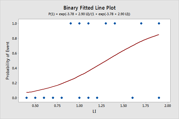
To illustrate, consider data published on n = 27 leukemia patients. The Leukemia Remission data set has a response variable of whether leukemia remission occurred (REMISS), which is given by a 1.
The predictor variables are cellularity of the marrow clot section (CELL), smear differential percentage of blasts (SMEAR), percentage of absolute marrow leukemia cell infiltrate (INFIL), percentage labeling index of the bone marrow leukemia cells (LI), the absolute number of blasts in the peripheral blood (BLAST), and the highest temperature before the start of treatment (TEMP).
The following gives the estimated logistic regression equation and associated significance tests from Minitab:
- Select Stat > Regression > Binary Logistic Regression > Fit Binary Logistic Model.
- Select "REMISS" for the Response (the response event for remission is 1 for this data).
- Select all the predictors as Continuous predictors.
- Click Options and choose Deviance or Pearson residuals for diagnostic plots.
- Click Graphs and select "Residuals versus order."
- Click Results and change "Display of results" to "Expanded tables."
- Click Storage and select "Coefficients."
This results in the following output:
Coefficients
| Term | Coef | SE Coef | 95% CI | Z-Value | P-Value | VIF |
|---|---|---|---|---|---|---|
| Constant | 64.3 | 75.0 | ( -82.7, 211.2) | 0.86 | 0.391 | |
| CELL | 30.8 | 52.1 | ( -71.4, 133.0) | 0.59 | 0.554 | 62.46 |
| SMEAR | 24.7 | 61.5 | ( -95.9, 145.3) | 0.40 | 0.688 | 434.42 |
| INFILL | -25.0 | 65.3 | ( - 152.9, 103.0) | -0.38 | 0.702 | 471.10 |
| LI | 4.36 | 2.66 | ( -0.85, 9.57) | 1.64 | 0.101 | 4.43 |
| Blast | -0.01 | 2.27 | ( -4.45, 4.43) | -0.01 | 0.996 | 4.18 |
| TEMP | -100.2 | 77.8 | (-252.6, 52.2) | -1.29 | 0.198 | 3.01 |
Wald Test
The Wald test is the test of significance for individual regression coefficients in logistic regression (recall that we use t-tests in linear regression). For maximum likelihood estimates, the ratio
\(\begin{equation*}
Z=\dfrac{\hat{\beta}_{i}}{\textrm{s.e.}(\hat{\beta}_{i})}
\end{equation*}\)
can be used to test \(H_{0} \colon \beta_{i}=0\). The standard normal curve is used to determine the \(p\)-value of the test. Furthermore, confidence intervals can be constructed as
\(\begin{equation*}
\hat{\beta}_{i}\pm z_{1-\alpha/2}\textrm{s.e.}(\hat{\beta}_{i}).
\end{equation*}\)
Estimates of the regression coefficients, \(\hat{\beta}\), are given in the Minitab output Coefficients table in the column labeled "Coef." This table also gives coefficient p-values based on Wald tests. The index of the bone marrow leukemia cells (LI) has the smallest p-value and so appears to be closest to a significant predictor of remission occurring. After looking at various subsets of the data, we find that a good model is one that only includes the labeling index as a predictor:
Coefficients
| Term | Coef | SE Coef | 95% CI | Z-Value | P-Value | VIF |
|---|---|---|---|---|---|---|
| Constant | -3.78 | 1.38 | ( -6.48, -1.08) | -2.74 | 0.006 | |
| LI | 2.90 | 1.19 | ( -0.57, 5.22) | 2.44 | 0.015 | 1.00 |
Regression Equation
p(1) = exp(Y')/(1 + exp(Y'))
Y' = -3.78 + 2.90 LI
Since we only have a single predictor in this model we can create a Binary Fitted Line Plot to visualize the sigmoidal shape of the fitted logistic regression curve:
Odds, Log Odds, and Odds Ratio
There are algebraically equivalent ways to write the logistic regression model:
The first is
\(\begin{equation}\label{logmod1}
\dfrac{\pi}{1-\pi}=\exp(\beta_{0}+\beta_{1}X_{1}+\ldots+\beta_{p-1}X_{p-1}),
\end{equation}\)
which is an equation that describes the odds of being in the current category of interest. By definition, the odds for an event is \(\pi\) / (1 - π) such that π is the probability of the event. For example, if you are at the racetrack and there is an 80% chance that a certain horse will win the race, then his odds are 0.80 / (1 - 0.80) = 4, or 4:1.
The second is
\(\begin{equation}\label{logmod2}
\log\biggl(\dfrac{\pi}{1-\pi}\biggr)=\beta_{0}+\beta_{1}X_{1}+\ldots+\beta_{p-1}X_{p-1},
\end{equation}\)
which states that the (natural) logarithm of the odds is a linear function of the X variables (and is often called the log odds). This is also referred to as the logit transformation of the probability of success, \(\pi\).
The odds ratio (which we will write as \(\theta\)) between the odds for two sets of predictors (say \(\textbf{X}_{(1)}\) and \(\textbf{X}_{(2)}\)) is given by
\(\begin{equation*}
\theta=\dfrac{(\pi/(1-\pi))|_{\textbf{X}=\textbf{X}_{(1)}}}{(\pi/(1-\pi))|_{\textbf{X}=\textbf{X}_{(2)}}}.
\end{equation*}\)
For binary logistic regression, the odds of success are:
\(\begin{equation*}
\dfrac{\pi}{1-\pi}=\exp(\textbf{X}\beta).
\end{equation*}\)
By plugging this into the formula for \(\theta\) above and setting \(\textbf{X}_{(1)}\) equal to \(\textbf{X}_{(2)}\) except in one position (i.e., only one predictor differs by one unit), we can determine the relationship between that predictor and the response. The odds ratio can be any nonnegative number. An odds ratio of 1 serves as the baseline for comparison and indicates there is no association between the response and predictor. If the odds ratio is greater than 1, then the odds of success are higher for higher levels of a continuous predictor (or for the indicated level of a factor). In particular, the odds increase multiplicatively by \(\exp(\beta_{j})\) for every one-unit increase in \(\textbf{X}_{j}\). If the odds ratio is less than 1, then the odds of success are less for higher levels of a continuous predictor (or for the indicated level of a factor). Values farther from 1 represent stronger degrees of association.
For example, when there is just a single predictor, \(X\), the odds of success are:
\(\begin{equation*}
\dfrac{\pi}{1-\pi}=\exp(\beta_0+\beta_1X).
\end{equation*}\)
If we increase \(X\) by one unit, the odds ratio is
\(\begin{equation*}
\theta=\dfrac{\exp(\beta_0+\beta_1(X+1))}{\exp(\beta_0+\beta_1X)}=\exp(\beta_1).
\end{equation*}\)
To illustrate, the relevant Minitab output from the leukemia example is:
Odd Ratios for Continuous Predictors
| Odds Ratio | 95% CI | |
|---|---|---|
| LI | 18.1245 | (1.7703, 185.5617) |
The odds ratio for LI of 18.1245 is calculated as \(\exp(2.89726)\) (you can view more decimal places for the coefficient estimates in Minitab by clicking "Storage" in the Regression Dialog and selecting "Coefficients"). The 95% confidence interval is calculated as \(\exp(2.89726\pm z_{0.975}*1.19)\), where \(z_{0.975}=1.960\) is the \(97.5^{\textrm{th}}\) percentile from the standard normal distribution. The interpretation of the odds ratio is that for every increase of 1 unit in LI, the estimated odds of leukemia remission are multiplied by 18.1245. However, since the LI appears to fall between 0 and 2, it may make more sense to say that for every .1 unit increase in L1, the estimated odds of remission are multiplied by \(\exp(2.89726\times 0.1)=1.336\). Then
- At LI=0.9, the estimated odds of leukemia remission is \(\exp\{-3.77714+2.89726*0.9\}=0.310\).
- At LI=0.8, the estimated odds of leukemia remission is \(\exp\{-3.77714+2.89726*0.8\}=0.232\).
- The resulting odds ratio is \(\dfrac{0.310}{0.232}=1.336\), which is the ratio of the odds of remission when LI=0.9 compared to the odds when L1=0.8.
Notice that \(1.336\times 0.232=0.310\), which demonstrates the multiplicative effect by \(\exp(0.1\hat{\beta_{1}})\) on the odds.
Likelihood Ratio (or Deviance) Test
The likelihood ratio test is used to test the null hypothesis that any subset of the \(\beta\)'s is equal to 0. The number of \(\beta\)'s in the full model is p, while the number of \(\beta\)'s in the reduced model is r. (Remember the reduced model is the model that results when the \(\beta\)'s in the null hypothesis are set to 0.) Thus, the number of \(\beta\)'s being tested in the null hypothesis is \(p-r\). Then the likelihood ratio test statistic is given by:
\(\begin{equation*}
\Lambda^{*}=-2(\ell(\hat{\beta}^{(0)})-\ell(\hat{\beta})),
\end{equation*}\)
where \(\ell(\hat{\beta})\) is the log-likelihood of the fitted (full) model and \(\ell(\hat{\beta}^{(0)})\) is the log-likelihood of the (reduced) model specified by the null hypothesis evaluated at the maximum likelihood estimate of that reduced model. This test statistic has a \(\chi^{2}\) distribution with \(p-r\) degrees of freedom. Minitab presents results for this test in terms of "deviance," which is defined as \(-2\) times log-likelihood. The notation used for the test statistic is typically \(G^2\) = deviance (reduced) – deviance (full).
This test procedure is analogous to the general linear F test for multiple linear regression. However, note that when testing a single coefficient, the Wald test and likelihood ratio test will not, in general, give identical results.
To illustrate, the relevant software output from the leukemia example is:
Deviance Table
| Source | DF | Adj Dev | Adj Mean | Chi-Square | P-Value |
|---|---|---|---|---|---|
| Regression | 1 | 8.299 | 8.299 | 8.30 | 0.004 |
| LI | 1 | 8.299 | 8.299 | 8.30 | 0.004 |
| Error | 25 | 26.073 | 1.043 | ||
| Total | 26 | 34.372 |
Since there is only a single predictor for this example, this table simply provides information on the likelihood ratio test for LI (p-value of 0.004), which is similar but not identical to the earlier Wald test result (p-value of 0.015). The Deviance Table includes the following:
- The null (reduced) model, in this case, has no predictors, so the fitted probabilities are simply the sample proportion of successes, \(9/27=0.333333\). The log-likelihood for the null model is \(\ell(\hat{\beta}^{(0)})=-17.1859\), so the deviance for the null model is \(-2\times-17.1859=34.372\), which is shown in the "Total" row in the Deviance Table.
- The log-likelihood for the fitted (full) model is \(\ell(\hat{\beta})=-13.0365\), so the deviance for the fitted model is \(-2\times-13.0365=26.073\), which is shown in the "Error" row in the Deviance Table.
- The likelihood ratio test statistic is therefore \(\Lambda^{*}=-2(-17.1859-(-13.0365))=8.299\), which is the same as \(G^2=34.372-26.073=8.299\).
- The p-value comes from a \(\chi^{2}\) distribution with \(2-1=1\) degrees of freedom.
When using the likelihood ratio (or deviance) test for more than one regression coefficient, we can first fit the "full" model to find deviance (full), which is shown in the "Error" row in the resulting full model Deviance Table. Then fit the "reduced" model (corresponding to the model that results if the null hypothesis is true) to find deviance (reduced), which is shown in the "Error" row in the resulting reduced model Deviance Table. For example, the relevant Deviance Tables for the Disease Outbreak example on pages 581-582 of Applied Linear Regression Models (4th ed) by Kutner et al are:
Full model
| Source | DF | Adj Dev | Adj Mean | Chi-Square | P-Value |
|---|---|---|---|---|---|
| Regression | 9 | 28.322 | 3.14686 | 28.32 | 0.001 |
| Error | 88 | 93.996 | 1.06813 | ||
| Total | 97 | 122.318 |
Reduced Model
| Source | DF | Adj Dev | Adj Mean | Chi-Square | P-Value |
|---|---|---|---|---|---|
| Regression | 4 | 21.263 | 5.3159 | 21.26 | 0.000 |
| Error | 93 | 101.054 | 1.06813 | ||
| Total | 97 | 122.318 |
Here the full model includes four single-factor predictor terms and five two-factor interaction terms, while the reduced model excludes the interaction terms. The test statistic for testing the interaction terms is \(G^2 = 101.054-93.996 = 7.058\), which is compared to a chi-square distribution with \(10-5=5\) degrees of freedom to find the p-value > 0.05 (meaning the interaction terms are not significant).
Alternatively, select the corresponding predictor terms last in the full model and request Minitab to output Sequential (Type I) Deviances. Then add the corresponding Sequential Deviances in the resulting Deviance Table to calculate \(G^2\). For example, the relevant Deviance Table for the Disease Outbreak example is:
| Source | DF | Seq Dev | Seq Mean | Chi-Square | P-Value |
|---|---|---|---|---|---|
| Regression | 9 | 28.322 | 3.1469 | 28.32 | 0.001 |
| --Age | 1 | 7.405 | 7.4050 | 7.40 | 0.007 |
| --Middle | 1 | 1.804 | 1.8040 | 1.80 | 0.179 |
| --Lower | 1 | 1.606 | 1.6064 | 1.61 | 0.205 |
| Sector | 1 | 10.448 | 10.4481 | 10.45 | 0.001 |
| Age*Middle | 1 | 4.570 | 4.5397 | 4.57 | 0.033 |
| Age*Lower | 1 | 1.015 | 1.0152 | 1.02 | 0.314 |
| Age*Sector | 1 | 1.120 | 1.1202 | 1.12 | 0.290 |
| Middle*Sector | 1 | 0.000 | 0.0001 | 0.00 | 0.993 |
| Lower*Sector | 1 | 0.353 | 0.3531 | 0.35 | 0.3552 |
| Error | 88 | 93.996 | 1.0681 | ||
| Total | 97 | 122.318 |
The test statistic for testing the interaction terms is \(G^2 = 4.570+1.015+1.120+0.000+0.353 = 7.058\), the same as in the first calculation.
Goodness-of-Fit Tests
The overall performance of the fitted model can be measured by several different goodness-of-fit tests. Two tests that require replicated data (multiple observations with the same values for all the predictors) are the Pearson chi-square goodness-of-fit test and the deviance goodness-of-fit test(analogous to the multiple linear regression lack-of-fit F-test). Both of these tests have statistics that are approximately chi-square distributed with c - p degrees of freedom, where c is the number of distinct combinations of the predictor variables. When a test is rejected, there is a statistically significant lack of fit. Otherwise, there is no evidence of a lack of fit.
By contrast, the Hosmer-Lemeshow goodness-of-fit test is helpful for unreplicated datasets or for datasets that contain just a few replicated observations. For this test, the observations are grouped based on their estimated probabilities. The resulting test statistic is approximately chi-square distributed with c - 2 degrees of freedom, where c is the number of groups (generally chosen to be between 5 and 10, depending on the sample size).
To illustrate, the relevant Minitab output from the leukemia example is:
Goodness-of-Fit Test
| Test | DF | Chi-square | P-Value |
|---|---|---|---|
| Deviance | 25 | 26.07 | 0.404 |
| Pearson | 25 | 23.93 | 0.523 |
| Hosmer-Lemeshow | 7 | 6.87 | 0.442 |
Since there is no replicated data for this example, the deviance and Pearson goodness-of-fit tests are invalid, so the first two rows of this table should be ignored. However, the Hosmer-Lemeshow test does not require replicated data so we can interpret its high p-value as indicating no evidence of lack of fit.
\(R^{2}\)
The calculation of \(R^{2}\) used in linear regression does not extend directly to logistic regression. One version of \(R^{2}\) used in logistic regression is defined as
\(\begin{equation*}
R^{2}=\dfrac{\ell(\hat{\beta_{0}})-\ell(\hat{\beta})}{\ell(\hat{\beta_{0}})-\ell_{S}(\beta)},
\end{equation*}\)
where \(\ell(\hat{\beta_{0}})\) is the log-likelihood of the model when only the intercept is included and \(\ell_{S}(\beta)\) is the log-likelihood of the saturated model (i.e., where a model is fit perfectly to the data). This \(R^{2}\) does go from 0 to 1 with 1 being a perfect fit. With unreplicated data, \(\ell_{S}(\beta)=0\), so the formula simplifies to:
\(\begin{equation*}
R^{2}=\dfrac{\ell(\hat{\beta_{0}})-\ell(\hat{\beta})}{\ell(\hat{\beta_{0}})}=1-\dfrac{\ell(\hat{\beta})}{\ell(\hat{\beta_{0}})}.
\end{equation*}\)
To illustrate, the relevant Minitab output from the leukemia example is:
Model Summary
| Deviance R-Sq |
Deviance R-Sq(adj) |
AIC |
|---|---|---|
| 24.14% | 21.23% | 30.07 |
Recall from above that \(\ell(\hat{\beta})=-13.0365\) and \(\ell(\hat{\beta}^{(0)})=-17.1859\), so:
\(\begin{equation*}
R^{2}=1-\dfrac{-13.0365}{-17.1859}=0.2414.
\end{equation*}\)
Note that we can obtain the same result by simply using deviances instead of log-likelihoods since the \(-2\) factor cancels out:
\(\begin{equation*}
R^{2}=1-\dfrac{26.073}{34.372}=0.2414.
\end{equation*}\)
Raw Residual
The raw residual is the difference between the actual response and the estimated probability from the model. The formula for the raw residual is
\(\begin{equation*}
r_{i}=y_{i}-\hat{\pi}_{i}.
\end{equation*}\)
Pearson Residual
The Pearson residual corrects for the unequal variance in the raw residuals by dividing by the standard deviation. The formula for the Pearson residuals is
\(\begin{equation*}
p_{i}=\dfrac{r_{i}}{\sqrt{\hat{\pi}_{i}(1-\hat{\pi}_{i})}}.
\end{equation*}\)
Deviance Residuals
Deviance residuals are also popular because the sum of squares of these residuals is the deviance statistic. The formula for the deviance residual is
\(\begin{equation*}
d_{i}=\pm\sqrt{2\biggl(y_{i}\log\biggl(\dfrac{y_{i}}{\hat{\pi}_{i}}\biggr)+(1-y_{i})\log\biggl(\dfrac{1-y_{i}}{1-\hat{\pi}_{i}}\biggr)\biggr)}.
\end{equation*}\)
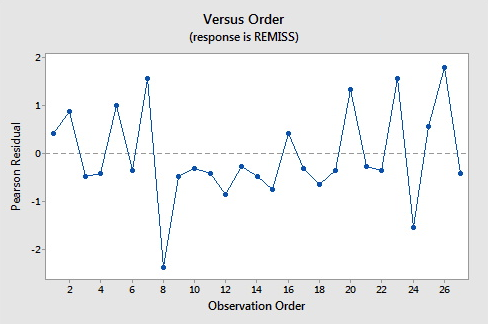
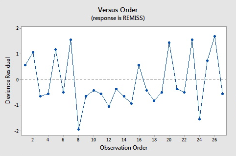
Here are the plots of the Pearson residuals and deviance residuals for the leukemia example. There are no alarming patterns in these plots to suggest a major problem with the model.
Hat Values
The hat matrix serves a similar purpose as in the case of linear regression – to measure the influence of each observation on the overall fit of the model – but the interpretation is not as clear due to its more complicated form. The hat values (leverages) are given by
\(\begin{equation*}
h_{i,i}=\hat{\pi}_{i}(1-\hat{\pi}_{i})\textbf{x}_{i}^{\textrm{T}}(\textbf{X}^{\textrm{T}}\textbf{W}\textbf{X})\textbf{x}_{i},
\end{equation*}\)
where W is an \(n\times n\) diagonal matrix with the values of \(\hat{\pi}_{i}(1-\hat{\pi}_{i})\) for \(i=1 ,\ldots,n\) on the diagonal. As before, we should investigate any observations with \(h_{i,i}>3p/n\) or, failing this, any observations with \(h_{i,i}>2p/n\) and very isolated.
Studentized Residuals
We can also report Studentized versions of some of the earlier residuals. The Studentized Pearson residuals are given by
\(\begin{equation*}
sp_{i}=\dfrac{p_{i}}{\sqrt{1-h_{i,i}}}
\end{equation*}\)
and the Studentized deviance residuals are given by
\(\begin{equation*}
sd_{i}=\dfrac{d_{i}}{\sqrt{1-h_{i, i}}}.
\end{equation*}\)
C and \(\bar{\textrm{C}}\)
C and \(\bar{\textrm{C}}\) are extensions of Cook's distance for logistic regression. C measures the overall change in fitted logits due to deleting the \(i^{\textrm{th}}\) observation for all points including the one deleted, while \(\bar{\textrm{C}}\) excludes the deleted point. They are defined by:
\(\begin{equation*}
\textrm{C}_{i}=\dfrac{p_{i}^{2}h _{i,i}}{p(1-h_{i,i})^{2}}
\end{equation*}\)
and
\(\begin{equation*}
\bar{\textrm{C}}_{i}=\dfrac{p_{i}^{2}h_{i,i}}{p(1-h_{i,i})}.
\end{equation*}\)
To illustrate, the relevant Minitab output from the leukemia example is:
Fits and Diagnostics for Unusual Observations
| Obs | Probability | Fit | SE Fit | 95% CI | Resid | Std Resid | Del Resid | HI |
|---|---|---|---|---|---|---|---|---|
| 8 | 0.000 | 0.849 | 0.139 | (0.403, 0.979) | -1.945 | -2.11 | -2.19 | 0.149840 |
Fits and Diagnostics for Unusual Observations
| Obs | Cook's D | DFITS | |
|---|---|---|---|
| 8 | 0.58 | -1.08011 | R |
R Large residual
The default residuals in this output (set under Minitab's Regression Options) are deviance residuals, so observation 8 has a deviance residual of \(-1.945\), a studentized deviance residual of \(-2.11\), a leverage (h) of \(0.149840\), and a Cook's distance (C) of 0.58.
DFDEV and DFCHI
DFDEV and DFCHI are statistics that measure the change in deviance and in Pearson's chi-square, respectively, that occurs when an observation is deleted from the data set. Large values of these statistics indicate observations that have not been fitted well. The formulas for these statistics are
\(\begin{equation*}
\textrm{DFDEV}_{i}=d_{i}^{2}+\bar{\textrm{C}}_{i}
\end{equation*}\)
and
\(\begin{equation*}
\textrm{DFCHI}_{i}=\dfrac{\bar{\textrm{C}}_{i}}{h_{i,i}}
\end{equation*}\)
13.2.1 - Further Logistic Regression Examples
13.2.1 - Further Logistic Regression ExamplesExample 15-1: STAT 200 Dataset
Students in STAT 200 at Penn State were asked if they have ever driven after drinking (the dataset unfortunately no longer available). They also were asked, “How many days per month do you drink at least two beers?” In the following discussion, \(\pi\) = the probability a student says “yes” they have driven after drinking. This is modeled using X = days per month of drinking two beers. Results from Minitab were as follows.
| Variable | Value | Count |
|---|---|---|
| DrivDrnk | Yes | 122 (Event) |
| No | 127 | |
| Total | 249 |
| 95% CI | |||||||
|---|---|---|---|---|---|---|---|
| Coef | SE Coef | Z | P | Odds Ratio | Lower | Upper | |
| Constant | -1.5514 | 0.2661 | -5.83 | 0.000 | |||
| DaysBeer | 0.19031 | 0.02946 | 6.46 | 0.000 | 1.21 | 1.14 | 1.28 |
Some things to note from the results are:
- We see that in the sample 122/249 students said they have driven after drinking. (Yikes!)
- Parameter estimates, given under Coef are \(\hat{\beta}_0\) = −1.5514, and \(\hat{\beta}_1\) = 0.19031.
- The model for estimating \(\pi\) = the probability of ever having driven after drinking is
\(\hat{\pi}=\dfrac{\exp(-1.5514+0.19031X)}{1+\exp(-1.5514+0.19031X)}\)
- The variable X = DaysBeer is a statistically significant predictor (Z = 6.46, P = 0.000).
We can also obtain a plot of the estimated probability of ever having driven under the influence (\(\pi\)) versus days per month of drinking at least two beers.
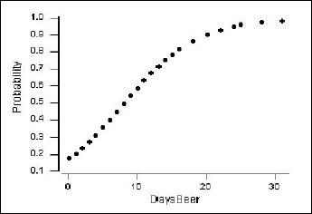
The vertical axis shows the probability of ever having driven after drinking. For example, if X = 4 days per month of drinking beer, then the estimated probability is calculated as:
\(\hat{\pi}=\dfrac{\exp(-1.5514+0.19031(4))}{1+\exp(-1.5514+0.19031(4))}=\frac{\exp(-0.79016)}{1+\exp(-0.79016)}=0.312\)
A few of these estimated probabilities are given in the following table:
| DaysBeer | 4 | 12 | 20 | 28 |
|---|---|---|---|---|
| \(\hat{\pi}\) | 0.312 | 0.675 | 0.905 | 0.97 |
In the results given above, we see that the estimate of the odds ratio is 1.21 for DaysBeer. This is given under Odds Ratio in the table of coefficients, standard errors, and so on. The sample odds ratio was calculated as \(e^{0.19031}\). The interpretation of the odds ratio is that for each increase of one day of drinking beer per month, the predicted odds of having ever driven after drinking are multiplied by 1.21.
Above we found that at X = 4, the predicted probability of ever driving after drinking is \(\hat{\pi}\) = 0.312. Thus when X = 4, the predicted odds of ever driving after drinking is 0.312/(1 − 0.312) = 0.453. To find the odds when X = 5, one method would be to multiply the odds at X = 4 by the sample odds ratio. The calculation is 1.21 × 0.453 = 0.549. (Another method is to just do the calculation as we did for X = 4.)
Notice also, that the results give a 95% confidence interval estimate of the odd ratio (1.14 to 1.28).
We now include Gender (male or female) as an x-variable (along with DaysBeer). Some Minitab results are given below. Under Gender, the row for male is explaining that the program created an indicator variable with a value of 1 if the student is male and a value of 0 if the student is female.
| 95% CI | |||||||
|---|---|---|---|---|---|---|---|
| Coef | SE Coef | Z | P | Odds Ratio | Lower | Upper | |
| Constant | -1.7736 | 0.2945 | -6.02 | 0.000 | |||
| DaysBeer | 0.18693 | 0.03004 | 6.22 | 0.000 | 1.21 | 1.14 | 1.28 |
|
Gender male |
0.6172 | 0.2954 | 2.09 | 0.037 | 1.85 | 1.04 | 3.31 |
Some things to note from the results are:
- The p-values are less than 0.05 for both DaysBeer and Gender. This is evidence that both x-variables are useful for predicting the probability of ever having driven after drinking.
- For DaysBeer, the odds ratio is still estimated to equal 1.21 to two decimal places (calculated as \(e^{0.18693}\)).
- For Gender, the odds ratio is 1.85 (calculated as \(e^{0.6172}\)). For males, the odds of ever having driven after drinking is 1.85 times the odds for females, assuming DaysBeer is held constant.
Finally, the results for testing with respect to the multiple logistic regression model are as follows:
Log-Likelihood = -139.981
Test that all slopes are zero: G = 65.125, DF = 2, P-Value = 0.000
Notice that since we have a p-value of 0.000 for this chi-square test, we, therefore, reject the null hypothesis that all of the slopes are equal to 0.
Example 15-2: Toxicity Dataset

An experiment is done to test the effect of a toxic substance on insects. The data originate from the textbook, Applied Linear Statistical Models by Kutner, Nachtsheim, Neter, & Li.
At each of six dose levels, 250 insects are exposed to the substance and the number of insects that die is counted (Toxicity data). We can use Minitab to calculate the observed probabilities as the number of observed deaths out of 250 for each dose level.
A binary logistic regression model is used to describe the connection between the observed probabilities of death as a function of dose level. Since the data is in event/trial format the procedure in Minitab is a little different to before:
- Select Stat > Regression > Binary Logistic Regression > Fit Binary Logistic Model
- Select "Response is in event/trial format"
- Select "Deaths" for Number of events, "SampSize" for Number of trials (and type "Death" for Event name if you like)
- Select Dose as a Continuous predictor
- Click Results and change "Display of results" to "Expanded tables"
- Click Storage and select "Fits (event probabilities)"
The Minitab output is as follows:
Coefficients
| Term | Coef | SE Coef | 95% CI | Z | P | VIF |
|---|---|---|---|---|---|---|
| Constant | -2.644 | 0.156 | (-2.950, -2.338) | -16.94 | 0.000 | |
| Dose | 0.6740 | 0.0391 | (0.5973, 0.7506) | 17.23 | 0.000 | 1.00 |
Odds Ratios for Continuous Predictors
| Term | Odds Ratio | 95% CI |
|---|---|---|
| Dose | 1.9621 | (1.8173, 2.1184) |
Thus
\(\hat{\pi}=\dfrac{\exp(-2.644+0.674X)}{1+\exp(-2.644+0.674X)}\)
where X = Dose and \(\hat{\pi}\) is the estimated probability the insect dies (based on the model).
Predicted probabilities of death (based on the logistic model) for the six dose levels are given below (FITS). These probabilities closely agree with the observed values (Observed p) reported.
Data Display
| Row | Dose | SampSize | Deaths | Observed P | FITS |
|---|---|---|---|---|---|
| 1 | 1 | 250 | 28 | 0.112 | 0.122423 |
| 2 | 2 | 250 | 53 | 0.212 | 0.214891 |
| 3 | 3 | 250 | 93 | 0.372 | 0.349396 |
| 4 | 4 | 250 | 126 | 0.504 | 0.513071 |
| 5 | 5 | 250 | 172 | 0.688 | 0.673990 |
| 6 | 6 | 250 | 197 | 0.788 | 0.802229 |
As an example of calculating the estimated probabilities, for Dose 1, we have
\(\hat{\pi}=\dfrac{\exp(-2.644+0.674(1))}{1+\exp(-2.644+0.674(1))}=0.1224\)
The odds ratio for Dose is 1.9621, the value under Odds Ratio in the output. It was calculated as \(e^{0.674}\). The interpretation of the odds ratio is that for every increase of 1 unit in dose level, the estimated odds of insect death are multiplied by 1.9621.
As an example of odds and odds ratio:
- At Dose = 1, the estimated odds of death is \(\hat{\pi}/(1− \hat{\pi})\) = 0.1224/(1−0.1224) = 0.1395.
- At Dose = 2, the estimated odds of death is \(\hat{\pi}/(1− \hat{\pi})\) = 0.2149/(1−0.2149) = 0.2737.
- The Odds Ratio = \(\dfrac{0.2737}{0.1395}\), which is the ratio of the odds of death when Dose = 2 compared to the odds when Dose = 1.
A property of the binary logistic regression model is that the odds ratio is the same for any increase of one unit in X, regardless of the specific values of X.