8.1 - Example on Birth Weight and Smoking
8.1 - Example on Birth Weight and SmokingExample 8-1: Birth weight and Smoking during pregnancy
Researchers (Daniel, 1999) interested in answering the above research question collected the following data (Birth and Smokers dataset) on a random sample of n = 32 births:
- Response (y): birth weight (Weight) in grams of baby
- Potential predictor \(\left(x_{1}\right)\colon\) Smoking status of mother (yes or no)
- Potential predictor \(\left(x_{2}\right)\colon\) length of gestation (Gest) in weeks
The distinguishing feature of this data set is that one of the predictor variables — Smoking — is a qualitative predictor. To be more precise, smoking is a "binary variable" with only two possible values (yes or no). The other predictor variable (Gest) is, of course, quantitative.
The scatter plot matrix:
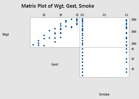
suggests, not surprisingly, that there is a positive linear relationship between the length of gestation and birth weight. That is, as the length of gestation increases, the birth weight of babies tends to increase. It is hard to see if any kind of (marginal) relationship exists between birth weight and smoking status, or between the length of gestation and smoking status.
The important question remains — after taking into account the length of gestation, is there a significant difference in the average birth weights of babies born to smoking and non-smoking mothers? A first-order model with one binary predictor and one quantitative predictor that helps us answer the question is:
\(y_i=(\beta_0+\beta_1x_{i1}+\beta_2x_{i2})+\epsilon_i\)
where:
- \(y_{i}\) is the birth weight of baby i
- \(x_{i1}\) is the length of gestation of baby i
- \(x_{i2}\) is a binary variable coded as a 1 if the baby's mother smoked during pregnancy and 0 if she did not
and the independent error terms \(\epsilon_i\) follow a normal distribution with mean 0 and equal variance \(\sigma^{2}\).
Notice that to include a qualitative variable in a regression model, we have to "code" the variable, that is, assign a unique number to each of the possible categories. We'll learn more about coding in the remainder of this lesson.
Using the sample data on n = 32 births, the plot of the estimated regression function looks like this:
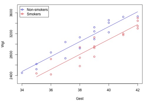
The blue circles represent the data on non-smoking mothers \(\left(x_2 = 0 \right) \), while the red circles represent the data on smoking mothers \(\left(x_{2} = 1\right)\). And, the blue line represents the estimated linear relationship between the length of gestation and birth weight for non-smoking mothers, while the red line represents the estimated linear relationship for smoking mothers.
At least in this sample of data, it appears as if the birth weights for non-smoking mothers are higher than that for smoking mothers, regardless of the length of gestation. A hypothesis test or confidence interval would allow us to see if this result extends to the larger population.
Did you expect the plot of the estimated regression equation to appear as two distinct lines? Let's consider this question. Minitab tells us that the estimated regression function is:
Regression Equation
Wgt = - 2390 + 143.10 Gest - 244.5 Smoke
Therefore, as illustrated in this screencast below, the estimated regression equation for non-smoking mothers (smoking = 0) is:
\(\widehat{Weight} = - 2390 + 143 Gest\)
and the estimated regression equation for smoking mothers (when smoking = 1) is:
\(\widehat{Weight} = - 2635 + 143 Gest\)
That is, we obtain two different parallel estimated lines (they are parallel because they have the same slope, 143). The difference between the two lines, –245, represents the difference in the average birth weights for a fixed gestation length for smoking and non-smoking mothers in the sample.
How would we answer the following set of research questions? (Do the procedures that appear in parentheses seem appropriate in answering the research question?)
- Is the baby's birth weight related to smoking during pregnancy, after taking into account the length of gestation? (Conduct a hypothesis test for testing whether the slope parameter for smoking is 0.)
- How is birth weight related to gestation, after taking into account a mother's smoking status? (Calculate and interpret a confidence interval for the slope parameter for gestation.)
Upon analyzing the data, the Minitab output:
Regression Analysis: Wgt versus Gest, Smoke
Analysis of Variance
| Source | DF | Adj SS | Adj MS | F-Value | P-Value |
|---|---|---|---|---|---|
| Regression | 2 | 3348720 | 1674360 | 125.45 | 0.000 |
| Gest | 1 | 3280270 | 3280270 | 245.76 | 0.000 |
| Smoke | 1 | 452881 | 452881 | 33.93 | 0.000 |
| Error | 29 | 387070 | 13347 | ||
| Lack-of-Fit | 12 | 52383 | 4365 | 0.22 | 0.994 |
| Pure Error | 17 | 334687 | 19687 | ||
| Total | 31 | 3735790 |
Model Summary
| S | R-sq | R-sq(adj) | R-sq(pred) |
|---|---|---|---|
| 115.530 | 89.64% | 88.92% | 87.6% |
Coefficients
| Term | Coef | SE Coef | T-Value | P-Value | VIF |
|---|---|---|---|---|---|
| Constant | -2390 | 349 | -6.84 | 0.000 | |
| Gest | 143.10 | 9.13 | 15.68 | 0.000 | 1.06 |
| Smoke | -244.5 | 42.0 | -5.83 | 0.000 | 1.06 |
Regression Equation
Wgt = - 2390 + 143.10 Gest - 244.5 Smoke
tells us that:
- A whopping 89.64% of the variation in the birth weights of babies is explained by the length of gestation and the smoking status of the mother.
- The P-values for the t-tests appearing in the table of estimates suggest that the slope parameters for Gest (P < 0.001) and Smoking (P < 0.001) are significantly different from 0.
- The P-value for the analysis of variance F-test (P < 0.001) suggests that the model containing the length of gestation and smoking status is more useful in predicting birth weight than not taking into account the two predictors.