13.1.1 - Weighted Least Squares Examples
13.1.1 - Weighted Least Squares ExamplesExample 13-1: Computer-Assisted Learning Dataset

The Computer-Assisted Learning New data was collected from a study of computer-assisted learning by n = 12 students.
| i | Responses | Cost |
|---|---|---|
| 1 | 16 | 77 |
| 2 | 14 | 70 |
| 3 | 22 | 85 |
| 4 | 10 | 50 |
| 5 | 14 | 62 |
| 6 | 17 | 70 |
| 7 | 10 | 55 |
| 8 | 13 | 63 |
| 9 | 19 | 88 |
| 10 | 12 | 57 |
| 11 | 18 | 81 |
| 12 | 11 | 51 |
The response is the cost of the computer time (Y) and the predictor is the total number of responses in completing a lesson (X). A scatterplot of the data is given below.
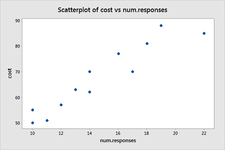
From this scatterplot, a simple linear regression seems appropriate for explaining this relationship.
First, an ordinary least squares line is fit to this data. Below is the summary of the simple linear regression fit for this data
Model Summary
| S | R-sq | R-sq(adj) | R-sq(pred) |
|---|---|---|---|
| 4.59830 | 88.91% | 87.80% | 81.27% |
Coefficients
| Term | Coef | SE Coef | T-Value | P-Value | VIF |
|---|---|---|---|---|---|
| Constant | 19.47 | 5.52 | 3.53 | 0.005 | |
| num.responses | 3.269 | 0.365 | 8.95 | 0.000 | 1.00 |
Regression Equation
cost = 19.47 + 3.269 num.responses
A plot of the residuals versus the predictor values indicates possible nonconstant variance since there is a very slight "megaphone" pattern:
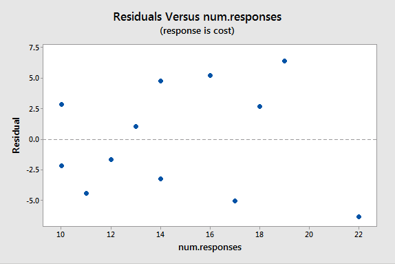
We will turn to weighted least squares to address this possibility. The weights we will use will be based on regressing the absolute residuals versus the predictor. In Minitab, we can use the Storage button in the Regression Dialog to store the residuals. Then we can use Calc > Calculator to calculate the absolute residuals. A plot of the absolute residuals versus the predictor values is as follows:
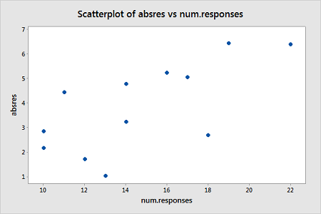
The weights we will use will be based on regressing the absolute residuals versus the predictor. Specifically, we will fit this model, use the Storage button to store the fitted values, and then use Calc > Calculator to define the weights as 1 over the squared fitted values. Then we fit a weighted least squares regression model by fitting a linear regression model in the usual way but clicking "Options" in the Regression Dialog and selecting the just-created weights as "Weights."
The summary of this weighted least squares fit is as follows:
Model Summary
| S | R-sq | R-sq(adj) | R-sq(pred) |
|---|---|---|---|
| 1.15935 | 89.51% | 88.46% | 83.87% |
Coefficients
| Term | Coef | SE Coef | T-Value | P-Value | VIF |
|---|---|---|---|---|---|
| Constant | 17.30 | 4.83 | 3.58 | 0.005 | |
| num.responses | 3.421 | 0.370 | 9.24 | 0.000 | 1.00 |
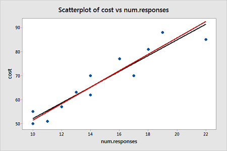
Notice that the regression estimates have not changed much from the ordinary least squares method. The following plot shows both the OLS fitted line (black) and WLS fitted line (red) overlaid on the same scatterplot.
A plot of the studentized residuals (remember Minitab calls these "standardized" residuals) versus the predictor values when using the weighted least squares method shows how we have corrected for the megaphone shape since the studentized residuals appear to be more randomly scattered about 0:
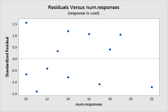
With weighted least squares, it is crucial that we use studentized residuals to evaluate the aptness of the model since these take into account the weights that are used to model the changing variance. The usual residuals don't do this and will maintain the same non-constant variance pattern no matter what weights have been used in the analysis.
Example 13-2: Market Share Data
Here we have market share data for n = 36 consecutive months (Market Share data). Let Y = market share of the product; \(X_1\) = price; \(X_2\) = 1 if the discount promotion is in effect and 0 otherwise; \(X_2\)\(X_3\) = 1 if both discount and package promotions in effect and 0 otherwise. The regression results below are for a useful model in this situation:
Coefficients
| Term | Coef | SE Coef | T-Value | P-Value | VIF |
|---|---|---|---|---|---|
| Constant | 3.196 | 0.356 | 8.97 | 0.000 | |
| Price | -0.334 | 0.152 | -2.19 | 0.036 | 1.01 |
| Discount | 0.3081 | 0.0641 | 4.80 | 0.000 | 1.68 |
| DiscountPromotion | 0.1762 | 0.0660 | 2.67 | 0.012 | 1.69 |
This model represents three different scenarios:
- Months in which there was no discount (and either a package promotion or not): X2 = 0 (and X3 = 0 or 1);
- Months in which there was a discount but no package promotion: X2 = 1 and X3 = 0;
- Months in which there was both a discount and a package promotion: X2 = 1 and X3 = 1.
So, it is fine for this model to break the hierarchy if there is no significant difference between the months in which there was no discount and no package promotion and months in which there was no discount but there was a package promotion.
A residual plot suggests nonconstant variance related to the value of \(X_2\):
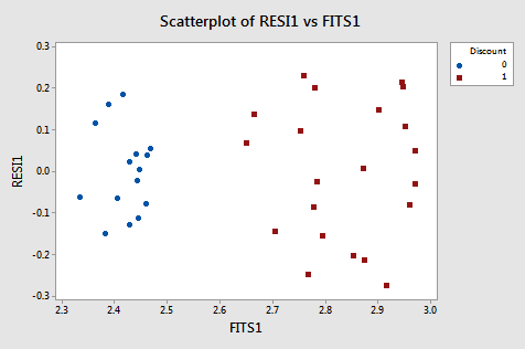
From this plot, it is apparent that the values coded as 0 have a smaller variance than the values coded as 1. The residual variances for the two separate groups defined by the discount pricing variable are:
| Discount | N | StDev | Variance | 95% CI for StDevs |
|---|---|---|---|---|
| 0 | 15 | 0.103 | 0.011 | (0.077, 0.158) |
| 1 | 21 | 0.164 | 0.027 | (0.136, 0.217) |
Because of this nonconstant variance, we will perform a weighted least squares analysis. For the weights, we use \(w_i=1 / \hat{\sigma}_i^2\) for i = 1, 2 (in Minitab use Calc > Calculator and define "weight" as ‘Discount'/0.027 + (1-‘Discount')/0.011 . The weighted least squares analysis (set the just-defined "weight" variable as "weights" under Options in the Regression dialog) is as follows:
Analysis of Variance
| Source | DF | Adj SS | Adj MS | F-Value | P-Value |
|---|---|---|---|---|---|
| Regression | 3 | 96.109 | 32.036 | 30.84 | 0.000 |
| Price | 1 | 4.688 | 4.688 | 4.51 | 0.041 |
| Discount | 1 | 23.039 | 23.039 | 22.18 | 0.000 |
| DiscountPromotion | 1 | 5.634 | 5.634 | 5.42 | 0.026 |
| Error | 32 | 33.246 | 1.039 | ||
| Total | 35 | 129.354 |
Coefficients
| Term | Coef | SE Coef | T-Value | P-Value | VIF |
|---|---|---|---|---|---|
| Constant | 3.175 | 0.357 | 8.90 | 0.000 | |
| Price | -0.325 | 0.153 | -2.12 | 0.041 | 1.01 |
| Discount | 0.3083 | 0.0655 | 4.71 | 0.000 | 2.04 |
| DiscountPromotion | 0.1759 | 0.0755 | 2.33 | 0.026 | 2.05 |
An important note is that Minitab’s ANOVA will be in terms of the weighted SS. When doing a weighted least squares analysis, you should note how different the SS values of the weighted case are from the SS values for the unweighted case.
Also, note how the regression coefficients of the weighted case are not much different from those in the unweighted case. Thus, there may not be much of an obvious benefit to using the weighted analysis (although intervals are going to be more reflective of the data).
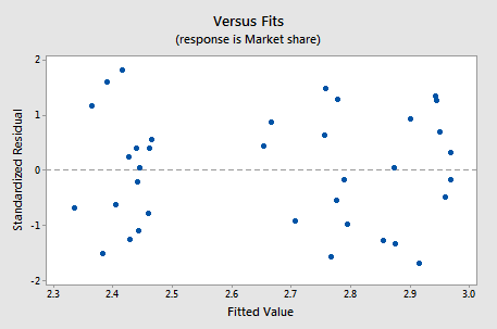
If you proceed with a weighted least squares analysis, you should check a plot of the residuals again. Remember to use the studentized residuals when doing so! For this example, the plot of studentized residuals after doing a weighted least squares analysis is given below and the residuals look okay (remember Minitab calls these standardized residuals).
Example 13-3: Home Price Dataset

The Home Price data set has the following variables:
Y = sale price of a home
\(X_1\) = square footage of the home
\(X_2\) = square footage of the lot
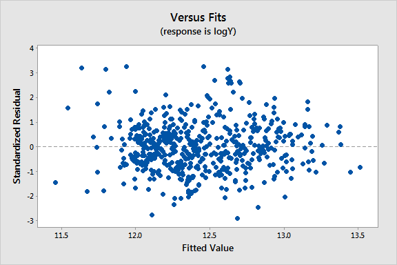
Since all the variables are highly skewed we first transform each variable to its natural logarithm. Then when we perform a regression analysis and look at a plot of the residuals versus the fitted values (see below), we note a slight “megaphone” or “conic” shape of the residuals.
| Term | Coef | SE Coeff | T-Value | P-Value | VIF |
|---|---|---|---|---|---|
| Constant | 1.964 | 0.313 | 6.28 | 0.000 | |
| logX1 | 1.2198 | 0.0340 | 35.87 | 0.000 | 1.05 |
| logX2 | 0.1103 | 0.0241 | 4.57 | 0.000 | 1.05 |
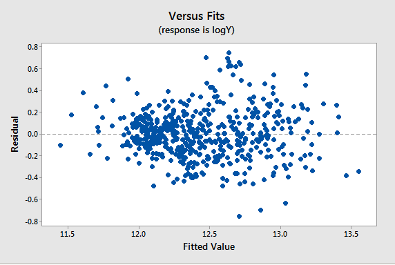
We interpret this plot as having a mild pattern of nonconstant variance in which the amount of variation is related to the size of the mean (which are the fits).
So, we use the following procedure to determine appropriate weights:
- Store the residuals and the fitted values from the ordinary least squares (OLS) regression.
- Calculate the absolute values of the OLS residuals.
- Regress the absolute values of the OLS residuals versus the OLS fitted values and store the fitted values from this regression. These fitted values are estimates of the error standard deviations.
- Calculate weights equal to \(1/fits^{2}\), where "fits" are the fitted values from the regression in the last step.
We then refit the original regression model but use these weights this time in a weighted least squares (WLS) regression.
Results and a residual plot for this WLS model:
| Term | Coef | SE Coeff | T-Value | P-Value | VIF |
|---|---|---|---|---|---|
| Constant | 2.377 | 0.284 | 8.38 | 0.000 | |
| logX1 | 1.2014 | 0.0336 | 35.72 | 0.000 | 1.08 |
| logX2 | 0.0831 | 0.0217 | 3.83 | 0.000 | 1.08 |
