Conducting a Hypothesis Test for the Population Correlation Coefficient P
Conducting a Hypothesis Test for the Population Correlation Coefficient PThere is one more point we haven't stressed yet in our discussion about the correlation coefficient r and the coefficient of determination r2 — namely, the two measures summarize the strength of a linear relationship in samples only. If we obtained a different sample, we would obtain different correlations, different r2 values, and therefore potentially different conclusions. As always, we want to draw conclusions about populations, not just samples. To do so, we either have to conduct a hypothesis test or calculate a confidence interval. In this section, we learn how to conduct a hypothesis test for the population correlation coefficient ρ (the Greek letter "rho").
Incidentally, where does this topic fit in among the four regression analysis steps?
- Model formulation
- Model estimation
- Model evaluation
- Model use
It's a situation in which we use the model to answer a specific research question, namely whether or not a linear relationship exists between two quantitative variables
In general, a researcher should use the hypothesis test for the population correlation ρ to learn of a linear association between two variables, when it isn't obvious which variable should be regarded as the response. Let's clarify this point with examples of two different research questions.
We previously learned that to evaluate whether or not a linear relationship exists between skin cancer mortality and latitude, we can perform either of the following tests:
- t-test for testing H0: β1= 0
- ANOVA F-test for testing H0: β1= 0
That's because it is fairly obvious that latitude should be treated as the predictor variable and skin cancer mortality as the response. Suppose we want to evaluate whether or not a linear relationship exists between a husband's age and his wife's age? In this case, one could treat the husband's age as the response:
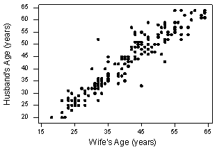
- Pearson correlation of HAge and WAge = 0.939
or one could treat wife's age as the response:
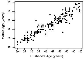
Pearson correlation of HAge and WAge = 0.939
In cases such as these, we answer our research question concerning the existence of a linear relationship by using the t-test for testing the population correlation coefficient H0: ρ = 0.
Let's jump right to it! We follow standard hypothesis test procedures in conducting a hypothesis test for the population correlation coefficient ρ. First, we specify the null and alternative hypotheses:
Null hypothesis H0: ρ = 0
Alternative hypothesis HA: ρ ≠ 0 or HA: ρ < 0 or HA: ρ > 0
Second, we calculate the value of the test statistic using the following formula:
Test statistic: \(t^*=\frac{r\sqrt{n-2}}{\sqrt{1-r^2}}\)
Third, we use the resulting test statistic to calculate the P-value. As always, the P-value is the answer to the question "how likely is it that we’d get a test statistic t* as extreme as we did if the null hypothesis were true?" The P-value is determined by referring to a t-distribution with n-2 degrees of freedom.
Finally, we make a decision:
- If the P-value is smaller than the significance level α, we reject the null hypothesis in favor of the alternative. We conclude "there is sufficient evidence at the α level to conclude that there is a linear relationship in the population between the predictor x and response y."
- If the P-value is larger than the significance level α, we fail to reject the null hypothesis. We conclude "there is not enough evidence at the α level to conclude that there is a linear relationship in the population between the predictor x and response y."
Let's perform the hypothesis test on the husband's age and wife's age data in which the sample correlation based on n = 170 couples is r = 0.939. To test H0: ρ = 0 against the alternative HA: ρ ≠ 0, we obtain the following test statistic:
\[t^*=\frac{r\sqrt{n-2}}{\sqrt{1-r^2}}=\frac{0.939\sqrt{170-2}}{\sqrt{1-0.939^2}}=35.39\]
To obtain the P-value, we need to compare the test statistic to a t-distribution with 168 degrees of freedom (since 170 - 2 = 168). In particular, we need to find the probability that we'd observe a test statistic more extreme than 35.39, and then, since we're conducting a two-sided test, multiply the probability by 2. Minitab helps us out here:
| Student's t distribution with 168 DF | |
|---|---|
| x | P ( X <= x ) |
| 35.3900 | 1.0000 |
The output tells us that the probability of getting a test statistic smaller than 35.39 is greater than 0.999. Therefore, the probability of getting a test statistic greater than 35.39 is less than 0.001. As illustrated in this ![]() , we multiply by 2 and determine that the P-value is less than 0.002. Since the P-value is small — smaller than 0.05, say — we can reject the null hypothesis. There is sufficient statistical evidence at the α = 0.05 level to conclude that there is a significant linear relationship between a husband's age and his wife's age.
, we multiply by 2 and determine that the P-value is less than 0.002. Since the P-value is small — smaller than 0.05, say — we can reject the null hypothesis. There is sufficient statistical evidence at the α = 0.05 level to conclude that there is a significant linear relationship between a husband's age and his wife's age.
Incidentally, we can let statistical software like Minitab do all of the dirty work for us. In doing so, Minitab reports:
| Pearson correlation of WAge and HAge= 0.939 | |
|---|---|
| P-Value = 0.000 |
It should be noted that the three hypothesis tests we learned for testing the existence of a linear relationship — the t-test for H0: β1= 0, the ANOVA F-test for H0: β1= 0, and the t-test for H0: ρ = 0 — will always yield the same results. For example, if we treat the husband's age ("HAge") as the response and the wife's age ("WAge") as the predictor, each test yields a P-value of 0.000... < 0.001:
| The regression equation is HAge= 3.59 + 0.967 WAge 170 cases used 48 cases contain missing values |
|||||
|---|---|---|---|---|---|
| Predictor | Coef | SE Coef | T | P | |
| Constant | 3.590 | 1.159 | 3.10 | 0.002 | |
| WAge | 0.96670 | 0.02742 | 35.25 | 0.000 | |
| S = 4.069 | R-Sq = 88.1% | R-sq(adj) = 88.0% | |||
| Analysis of Variance | |||||
| Source | DF | SS | MS | F | P |
| Regression | 1 | 20577 | 20577 | 1242.51 | 0.000 |
| Error | 168 | 2782 | 17 | ||
| Total | 169 | 23359 | |||
| Pearson correlation of WAge and HAge = 0.939 P-Value = 0.000 |
|||||
And similarly, if we treat the wife's age ("WAge") as the response and the husband's age ("HAge") as the predictor, each test yields of P-value of 0.000... < 0.001:
| The regression equation is WAge= 1.57 + 0.911 HAge 170 cases used 48 cases contain missing values |
|||||
|---|---|---|---|---|---|
| Predictor | Coef | SE Coef | T | P | |
| Constant | 1.574 | 1.150 | 1.37 | 0.173 | |
| WAge | 0.91124 | 0.02585 | 35.25 | 0.000 | |
| S = 3.951 | R-Sq = 88.1% | R-sq(adj) = 88.0% | |||
| Analysis of Variance | |||||
| Source | DF | SS | MS | F | P |
| Regression | 1 | 19396 | 19396 | 1242.51 | 0.000 |
| Error | 168 | 2623 | 17 | ||
| Total | 169 | 22019 | |||
| Pearson correlation of WAge and HAge = 0.939 P-Value = 0.000 |
|||||
Technically, then, it doesn't matter what test you use to obtain the P-value. You will always get the same P-value. But, you should report the results of the test that make sense for your particular situation:
- If one of the variables can be clearly identified as the response, report that you conducted a t-test or F-test results for testing H0: β1 = 0. (Does it make sense to use x to predict y?)
- If it is not obvious which variable is the response, report that you conducted a t-test for testing H0: ρ = 0. (Does it only make sense to look for an association between x and y?)
One final note ... as always, we should clarify when it is okay to use the t-test for testing H0: ρ = 0? The guidelines are a straightforward extension of the "LINE" assumptions made for the simple linear regression model. It's okay:
- When it is not obvious which variable is the response.
- When the (x, y) pairs are a random sample from a bivariate normal population.
- For each x, the y's are normal with equal variances.
- For each y, the x's are normal with equal variances.
- Either, y can be considered a linear function of x.
- Or, x can be considered a linear function of y.
- The (x, y) pairs are independent