3.1 - The Research Questions

In this lesson, we are concerned with answering two different types of research questions. Our goal here — and throughout the practice of statistics — is to translate the research questions into reasonable statistical procedures.

Let's take a look at examples of the two types of research questions we learn how to answer in this lesson:

1. What is the mean weight, \(\mu\), of all American women, aged 18-24?

If we wanted to estimate \(\mu\), what would be a good estimate? It seems reasonable to calculate a confidence interval for \(\mu\) using \(\bar{y}\), the average weight of a random sample of American women, aged 18-24.

2. What is the weight, y, of an individual American woman, aged 18-24?

If we want to predict y, what would be a good prediction? It seems reasonable to calculate a "prediction interval" for y using, again, \(\bar{y}\), the average weight of a random sample of American women, aged 18-24.

A person's weight is, of course, highly associated with the person's height. In answering each of the above questions, we likely could do better by taking into account a person's height. That's where an estimated regression equation becomes useful.

Here are some weight and height data from a sample of n = 10 people, (Student Height and Weight data):

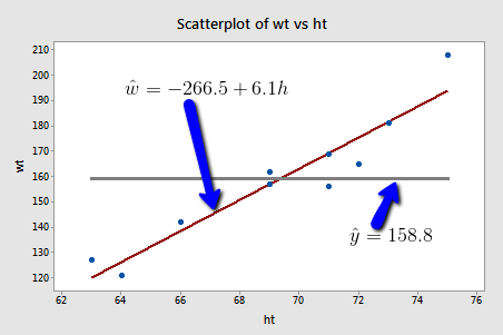
If we used the average weight of the 10 people in the sample to estimate \(\mu\), we would claim that the average weight of all American women aged 18-24 is 158.8 pounds regardless of the height of the women. Similarly, if we used the average weight of the 10 people in the sample to predict y, we would claim that the weight of an individual American woman aged 18-24 is 158.8 pounds regardless of the woman's height.

On the other hand, if we used the estimated regression equation to estimate \(\mu\), we would claim that the average weight of all American women aged 18-24 who are only 64 inches tall is -266.5 + 6.1(64) = 123.9 pounds. Similarly, we would predict that the weight y of an individual American woman aged 18-24 who is only 64 inches tall is 123.9 pounds. This example makes it clear that we get significantly different (and better!) answers to our research questions when we take into account a person's height.

Let's make it clear that it is one thing to estimate \(\mu_{Y}\)and yet another thing to predict y. (Note that we subscript \(\mu\) with Y to make it clear that we are talking about the mean of the response Y not the mean of the predictor x.)

Let's return to our example in which we consider the potential relationship between the predictor "high school GPA" and the response "college entrance test score."

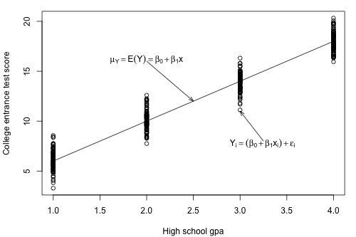
For this example, we could ask two different research questions concerning the response:

• What is the mean college entrance test score for the subpopulation of students whose high school GPA is 3? (Answering this question entails estimating the mean response \(\mu_{Y}\) when x = 3.)
• What college entrance test score can we predict for a student whose high school GPA is 3? (Answering this question entails predicting the response \(y_{\text{new}}\) when x = 3.)

The two research questions can be asked more generally:

• What is the mean response \(\mu_{Y}\) when the predictor value is \(x_{h}\)?
• What value will a new response \(y_{\text{new}}\) be when the predictor value is \(x_{h}\)?

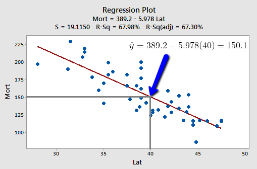
Let's take a look at one more example, namely, the one concerning the relationship between the response "skin cancer mortality" and the predictor "latitude" (Skin Cancer data). Again, we could ask two different research questions concerning the response:

• What is the expected (mean) mortality rate due to skin cancer for all locations at 40 degrees north latitude?
• What is the predicted mortality rate for one individual location at 40 degrees north, say at Chambersburg, Pennsylvania?

At some level, answering these two research questions is straightforward. Both just involve using the estimated regression equation:

That is, \(\hat{y}_h=b_0+b_1x_h\) is the best answer to each research question. It is the best guess of the mean response at \(x_{h}\), and it is the best guess of a new response at \(x_{h}\):

• Our best estimate of the mean mortality rate due to skin cancer for all locations at 40 degrees north latitude is 389.19 - 5.97764(40) = 150 deaths per 10 million people.
• Our best prediction of the mortality rate due to skin cancer in Chambersburg, Pennsylvania is 389.19 - 5.97764(40) = 150 deaths per 10 million people.

The problem with the answers to our two research questions is that we'd have obtained a completely different answer if we had selected a different random sample of data. As always, to be confident in the answer to our research questions, we should put an interval around our best guesses. We learn how to do this in the next two sections. That is, we first learn a "confidence interval for \(\mu_Y\) " and then a "prediction interval for \(y_{\text{new}}\)."