8.7 - Leaving an Important Interaction Out of a Model
8.7 - Leaving an Important Interaction Out of a ModelImpact of Removing a Necessary Interaction Term out of the Model
Before we take a look at another example of a regression model containing interaction terms, let's take a little detour to explore the impact of leaving a necessary interaction term out of the model. To do so, let's consider some contrived data for which there is a response y and two predictors —one quantitative predictor x, and one qualitative predictor that takes on values 0 or 1. Looking at a plot of the data:
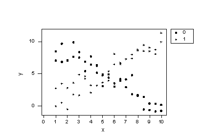
consider two questions:
-
Does the plot suggest that x is related to y? Sure! For the 0 group, as x increases, y decreases, while for the 1 group, as x increases, y also increases.
-
Does the plot suggest there is a treatment effect? Yes! If you look at any one particular x value, say 1 for example, the mean response y is about 8 for the 0 group and about 2 for the 1 group. In this sense, there is a treatment effect.
As we now know, the answer to the first question suggests that the effect of x on y depends on the group. That is, the group and x appear to interact. Therefore, our regression model should contain an interaction term between the two predictors. But, let's see what happens if we ignore our intuition and don't add the interaction term! That is, let's formulate our regression model as:
\(y_i=(\beta_0+\beta_1x_{i1}+\beta_2x_{i2})+\epsilon_i\)
where:
- \(y_i\) is the response
- \(x_{i1}\) is the quantitative predictor you want to "adjust for "
- \(x_{i2}\) is the qualitative group predictor, where 0 denotes the first group and 1 denotes the second group
and the independent error terms \(\epsilon_{i}\) follow a normal distribution with mean 0 and equal variance \(\sigma^{2}\).
Now, let's see what conclusions we draw when we fit our contrived data to our formulated model with no interaction term:
The Regression equation is y = 4.55 - 0.025 x + 1.10 group
| Predictor | Coef | SE Coef | T | P |
|---|---|---|---|---|
| Constant | 4.5492 | 0.8665 | 5.25 | 0.000 |
| x | -0.0276 | 0.1288 | -0.21 | 0.831 |
| group | 1.0959 | 0.7056 | 1.55 | 0.125 |
Analysis of Variance
| Source | DF | SS | MS | F | P |
|---|---|---|---|---|---|
| Regression | 2 | 23.255 | 11.628 | 1.23 | 0.298 |
| Residual Error | 73 | 690.453 | 9.458 | ||
| Total | 75 | 713.709 |
| Source | DF | Seq SS |
|---|---|---|
| x | 1 | 0.435 |
| group | 1 | 22.820 |
Consider our two research questions:
-
Is x related to y? Minitab reports that the P-value for testing \(H_0 \colon \beta_1 = 0 \text{ is } 0.831\). There is insufficient evidence at the 0.05 level to conclude that x is related to y. What?! This conclusion contradicts what we'd expect from the plot.
-
Is there a treatment effect? Minitab reports that the P-value for testing \(H_0 \colon \beta_2 = 0 \text{ is } 0.125\). There is insufficient evidence at the 0.05 level to conclude that there is a treatment effect. Again, this conclusion contradicts what we'd expect from the plot.
A side note. By conducting the above two tests independently, we increase our chance of making at least one Type I error. Since we are interested in answering both research questions, we could minimize our chance of making a Type I error by conducting the partial F-test for testing, \(H_0 \colon \beta_1 = \beta_2 = 0\), that is, that both parameters are simultaneously zero.
Now, let's try to understand why our conclusions don't agree with our intuition based on the plot. If we plug the values 0 and 1 into the group variable of the estimated regression equation we obtain two parallel lines —one for each group.
A plot of the resulting estimated regression functions:
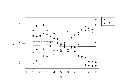
suggest that the lines don't fit the data very well. By leaving the interaction term out of the model, we have forced the "best fitting lines" to be parallel, when they clearly shouldn't be. The residuals versus fits plot:
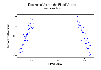
provides further evidence that our formulated model does not fit the data well. We now know that the resulting cost is conclusions that just don't make sense.
Let's analyze the data again, but this time with a more appropriately formulated model. Consider the regression model with the interaction term:
\(y_i=(\beta_0+\beta_1x_{i1}+\beta_2x_{i2}+\beta_{12}x_{i1}x_{i2})+\epsilon_i\)
where:
- \(y_i\) is the response
- \(x_{i1}\) is the quantitative predictor you want to "adjust for "
- \(x_{i2}\) is the qualitative group predictor, where 0 denotes the first group and 1 denotes the second group
- \(x_{i1}\)\(x_{i2}\) is the "missing" interaction term
and the independent error terms \(\epsilon_{i}\) follow a normal distribution with mean 0 and equal variance \(\sigma^{2}\).
Upon fitting the data to the model with an interaction term, Minitab reports:
Regression Equation
y = 10.1 - 1.04 x - 10.1 group + 2.03 groupxIf we now plug the values 0 and 1 into the group variable of the estimated regression equation we obtain two intersecting lines —one for each group:
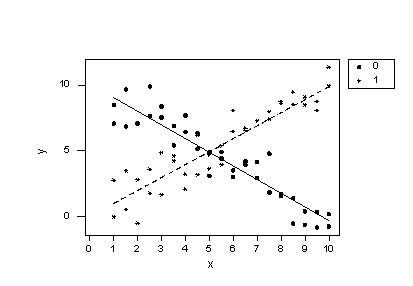
Wow —what a difference! Our formulated regression model now allows the slopes of the two lines to be different. As a result, the lines do a much better job of summarizing the trend in the data. The residuals versus fits plot is about as good as it gets!
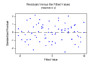
The plot provides further evidence that the model with the interaction term does a good job of describing the data.
Okay, so the model with the interaction term does a better job of describing the data than the model with no interaction term. Does it also provide answers to our research questions that make sense?
Let's first consider the question "does the effect of x on response y depend on the group?" That is, is there an interaction between x and the group? The Minitab output:
Regression Equation
y = 10.1 - 1.04 x - 10.1 group + 2.03 groupx
| Predictor | Coef | SE Coef | T | P |
|---|---|---|---|---|
| Constant | 10.1401 | 0.4320 | 23.47 | 0.000 |
| x | -1.04416 | 0.07031 | -14.85 | 0.000 |
| group | -10.0859 | 0.6110 | -16.51 | 0.000 |
| groupx | 2.03307 | 0.09944 | 20.45 | 0.000 |
| Model Summary | ||
|---|---|---|
| S = 1.187 | R-Sq = 85.8% | R-Sq(adj) = 85.2% |
Analysis of Variance
| Source | DF | SS | MS | F | P |
|---|---|---|---|---|---|
| Regression | 3 | 612.26 | 204.09 | 144.84 | 0.000 |
| Residual Error | 72 | 101.45 | 1.41 | ||
| Total | 75 | 713.71 |
tells us that the P-value for testing \(H_0 \colon \beta_{12} = 0 \text{ is } < 0.001\). There is strong evidence at the 0.05 level to reject the null hypothesis and conclude that there is indeed an interaction between x and the group. Aha —our formulated model and resulting analysis yielded a conclusion that makes sense!
Now, what about the research questions "is x related to y?" and "is there a treatment effect?" Because there is an interaction between x and the group, it doesn't make sense to talk about the effect of x on y without taking into account the group. And, it doesn't make sense to talk about differences in the two groups without taking into account x. That is, neither of these two research questions makes sense in the presence of the interaction. This is why you'll often hear statisticians say "never interpret the main effect in the presence of an interaction."
In short, the moral of the story of this little detour that we took is that if we leave an important interaction term out of our model, our analysis can lead us to make erroneous conclusions.