3.2 - Assumptions and Diagnostics
3.2 - Assumptions and DiagnosticsBefore we draw any conclusions about the significance of the model, we need to make sure we have a "valid" model. Like any other statistical procedure, the ANOVA has assumptions that must be met. Failure to meet these assumptions means any conclusions drawn from the model are not to be trusted.
Assumptions
So what are these assumptions being made to employ the ANOVA model? The errors are assumed to be independent and identically distributed (iid) with a normal distribution having a mean of 0 and unknown equal variance.
As the model residuals serve as estimates of the unknown error, diagnostic tests to check for validity of model assumptions are based on residual plots, and thus, the implementation of diagnostic tests is also called ‘Residual Analysis’.
Diagnostic Tests
Most useful is the residual vs. predicted value plot, which identifies the violations of zero mean and equal variance. Residuals are also plotted against the treatment levels to examine if the residual behavior differs among treatments. The normality assumption is checked by using a normal probability plot.
Residual plots can help identify potential outliers, and the pattern of residuals vs. fitted values or treatments may suggest a transformation of the response variable. Lesson 4: SLR Model Assumptions of STAT 501 online notes discuss various diagnostic procedures in more detail.
There are other various statistical tests to check the validity of these assumptions, but some may not be that useful. For example, Bartlett’s test for homogeneity is too sensitive and indicates that problems exist when they do not. It turns out that the ANOVA is very robust and is not overly affected by minor violations of these assumptions. In practice, a good deal of common sense and the visual inspection of the residual plots are sufficient to determine if serious problems exist.
Here are common patterns that you may encounter in the residual analysis (i.e. plotting residuals, \(e\) against the predicted values, \(\hat{y}\)). Figure (a) shows the prototype plot when the ANOVA model is appropriate for data. The residuals are scattered randomly around mean zero and variability is constant (i.e. within the horizontal bands) for all groups.
Figure (b) suggests that although the variance is constant, there are some trends in the response that is not explained by a linear model. Using figure (c), we can depict that the linear model is appropriate as the central trend in data is a line. However, the megaphone patterns in figure (c) suggest that variance is not constant.
In figure (d), we are plotting residuals against the order of the observations. The order-related trend depicts a prototype situation where the errors are not independent. In other words, errors that are near to each other in the sequence might be correlated with each other.
Alert!
A common problem encountered in ANOVA is when the variance of treatment levels is not equal (heterogeneity of variance). If the variance is increasing in proportion to the mean (panel (c) in the figure above), a logarithmic transformation of Y can 'stabilize' the variances. If the residuals vs. predicted values instead show a curvilinear trend (panel (b) in the figure above), then a quadratic or other transformation may help. Since finding the correct transformation can be challenging, the Box-Cox method is often used to identify the appropriate transformation, given in terms of \(\lambda\) as shown below.
\(y_i^{(\lambda)} = \begin{cases} \frac{y_i^\lambda - 1}{\lambda},& \text{if } \lambda \neq 0,\\ \ln y_i, & \text{if } \lambda = 0 \end{cases}\)
Some \(\lambda\) values result some common transformations.
| \(\lambda\) | \(Y^\lambda\) | Transformation |
|---|---|---|
| 2 | \(Y^2\) | Square |
| 1 | \(Y^1\) | Original (No transform) |
| 1/2 | \(\sqrt{Y}\) | Square Root |
| 0 | \(log(Y)\) | Logarithm |
| -1/2 | \(\frac{1}{\sqrt{Y}}\) | Reciprocal Square Root |
| -1 | \(\frac{1}{Y}\) | Reciprocal |
Using Technology
The Box-Cox procedure in SAS is more complicated in a general setting. It is done through the Transreg procedure, by obtaining the ANOVA solution with regression which first requires coding the treatment levels with effect coding discussed in Lesson 4.
However, for one-way ANOVA (ANOVA with only one factor) we can use the SAS Transreg procedure without much hassle. Suppose we have SAS data as follows.
| Obs | Treatment | ResponseVariable |
|---|---|---|
| 1 | A | 12 |
| 2 | A | 23 |
| 3 | A | 34 |
| 4 | B | 45 |
| 5 | B | 56 |
| 6 | B | 67 |
| 7 | C | 14 |
| 8 | C | 25 |
| 9 | C | 36 |
We can use the following SAS commands to run the Box-Cox analysis.
proc transreg data=boxcoxSimData;
model boxcox(ResponseVariable)=class(Treatment);
run;
This would generate an output as follows, which suggests a transformation using \(\lambda=1\) (i.e. no transformation).
To run the Box-Cox procedure in Minitab, set up the data (Simulated Data), as a stacked format (a column with treatment (or trt combination) levels, and the second column with the response variable.
| Treatment | Response Variable |
|---|---|
| A | 12 |
| A | 23 |
| A | 34 |
| B | 45 |
| B | 56 |
| B | 67 |
| C | 14 |
| C | 25 |
| C | 36 |
-
On the Minitab toolbar, choose
Stat > Control Charts > Box-Cox Transformation
-
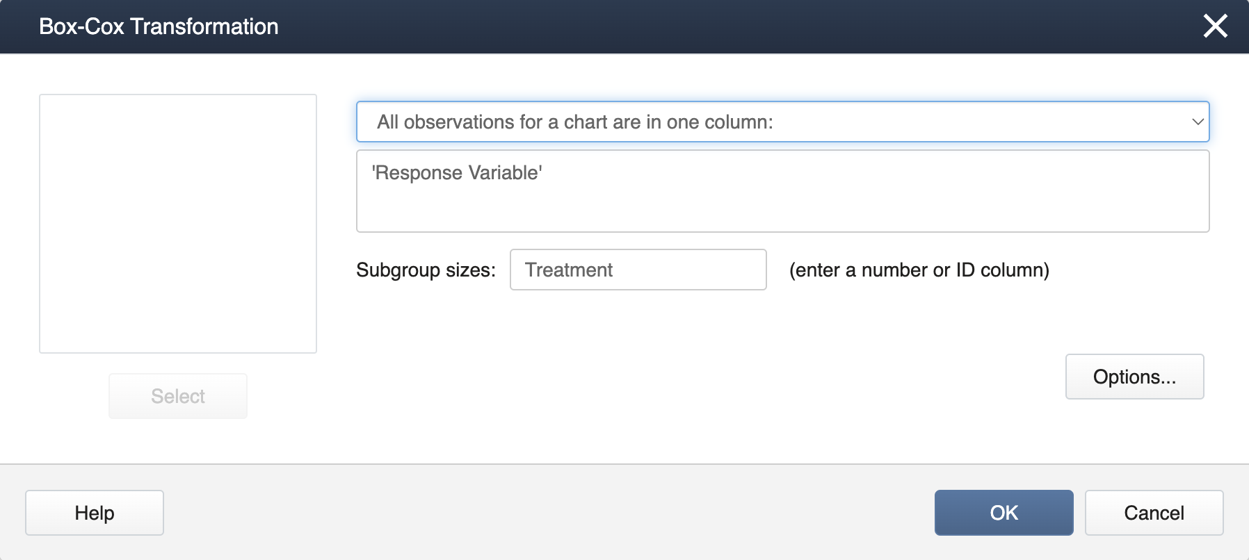
Place “Response Variable” and “Treatment” in the boxes as shown below.
-
Click OK to finish. You will get an output like this:
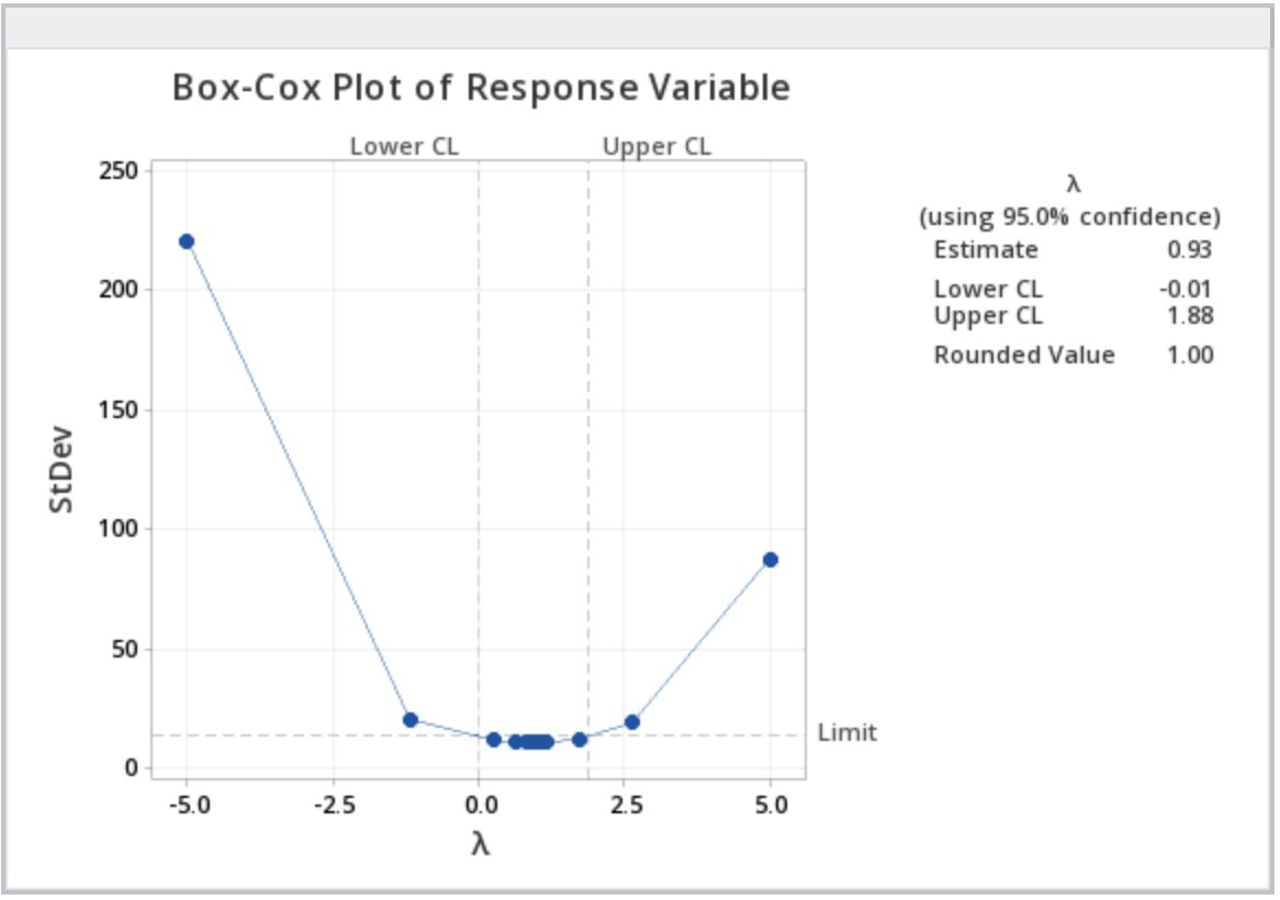
In the upper right-hand box, the rounded value for \(\lambda\) is given from which the appropriate transformation of the response variable can be found using the chart above. Note, with a \(\lambda\) of 1, no transformation is recommended.
First, load and attach the simulated data in R. Note that simulated data are in the stacked format (a column with treatment levels and a column with the response variable).
setwd("~/path-to-folder/")
simulated_data<-read.table("simulated_data.txt",header=T,sep ="\t")
attach(simulated_data)
Then we install and load the package AID and perform the Box-Cox procedure.
install.packages("AID")
library(AID)
boxcoxfr(Response_Variable,Treatment)
  Box-Cox power transformation
---------------------------------------------------------------------

  lambda.hat : 0.93


  Shapiro-Wilk normality test for transformed data (alpha = 0.05)
-------------------------------------------------------------------
  Level statistic   p.value Normality
1     A 0.9998983 0.9807382       YES
2     B 0.9999840 0.9923681       YES
3     C 0.9999151 0.9824033       YES


  Bartlett's homogeneity test for transformed data (alpha = 0.05)
-------------------------------------------------------------------
  Level   statistic   p.value Homogeneity
1   All 0.008271728 0.9958727         YES
---------------------------------------------------------------------
From the output, we can see that the \(\lambda\) value for the transformation is 0.93. Since this value is very close to 1 we can use \(\lambda=1\) (no transformation). In addition, from the output, we can see that normality exists in all 3 levels (Shapiro-Wilk test) and we have the same variance (Bartlett's test).
As an alternative method, we can use the boxcox function from the package MASS. The boxcox function produces a plot illustrating the 95% CI.
library(MASS)
Box_Cox_Plot<-boxcox(aov(Response.Variable~Treatment),lambda=seq(-3,3,0.01))
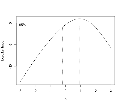
Since \(\lambda=1\) is within the CI, there is no need for transformation. We can also obtain the MLE \(\lambda\) (0.93) as follows.
lambda<-Box_Cox_Plot$x[which.max(Box_Cox_Plot$y)]
lambda
[1] 0.93
We conclude our analysis and detach the dataset.
detach(simulated_data)