6: Random Effects and Introduction to Mixed Models
6: Random Effects and Introduction to Mixed ModelsOverview
So far in our discussion of treatment designs, we have assumed (though unstated) that the treatment levels were chosen intentionally by the researcher dictated by their specific interests. In this situation, the scope of inference is limited to the specific (or fixed) treatment levels used in the study. However in practice, this is not always the case. Sometimes treatment levels may be a (random) sample of possible levels, and the scope of inference should be to a larger population of all possible levels.
If it is clear that the researcher is interested in comparing specific, chosen levels of treatment, that treatment is called a fixed effect. On the other hand, if the levels of the treatment are a sample from a larger population of possible levels, then the treatment is called a random effect.
Objectives
- Extend the treatment design to include random effects.
- Understand the basic concepts of random-effects models.
- Calculate and interpret the intraclass correlation coefficient.
- Combining fixed and random effects in the mixed model.
- Work with mixed models that include both fixed and random effects.
6.1 - Random Effects
6.1 - Random EffectsWhen a treatment (or factor) is a random effect, the model specifications as well as the relevant null and alternative hypotheses will have to be changed.
Recall the cell means model for the fixed effect case (from Lesson 4) which has the model equation
\(Y_{ij}=\mu_i+\epsilon_{ij}\)
where \(\mu_i\) are parameters for the treatment level means. For the single factor random effects model we have a very similar equation
\(Y_{ij}=\mu_i+\epsilon_{ij}\)
however, here \(\mu_i\) and \(\epsilon_{ij}\) are both independent random variables such that \(\mu_i \overset{iid}{\sim} \mathcal{N}\left(\mu, \sigma^2_{\mu}\right)\) and \(\epsilon_{ij} \overset{iid}{\sim} \mathcal{N}\left(0, \sigma_{\epsilon}^2\right)\) with \(i=1,2,...,T\), and \(j=1,2,...n_i\) where \(n_i \equiv n\) if the design is balanced.
The random effects ANOVA model is similar in appearance to the fixed effects ANOVA model. However, the treatment mean \(\mu_i\)'s are constant in the fixed-effect ANOVA model whereas in the random-effects ANOVA model the treatment mean \(\mu_i\)'s are random variables. Notice that the expected mean response in the random effects model stated above is the same at every treatment level and equals \(\mu\).
\(E\left(Y_{ij}\right) = E\left(\mu_i + \epsilon_{ij}\right) = E\left(\mu_i\right) + E\left(\epsilon_{ij}\right) = \mu \)
The variance of the response variable (say \(\sigma^2_{Y}\)) in the random effects model can be partitioned as
\(\sigma^2_{Y} = V\left(Y_{ij}\right) = V\left(\mu_i + \epsilon_{ij}\right) = V\left(\mu_i\right) + V\left(\epsilon_{ij}\right) = \sigma _{\mu}^{2}+\sigma_{\epsilon}^2\)
since \(\mu_i\) and \(\epsilon_{ij}\) are both independent random variables.
Similar to fixed effects ANOVA model, we can express the random effects ANOVA model using the factor effect representation, using \(\tau_i = \mu_i -\mu\). Therefore the factor effects representation of the random effects ANOVA model would be
\(Y_{ij} = \mu + \tau_i+\epsilon_{ij}\)
where \(\mu\) is a constant overall mean, \(\tau_i\) and \(\epsilon_{ij}\) are independent random variables such that \(\tau_i \overset{iid}{\sim} \mathcal{N}\left(0, \sigma^2_{\mu}\right)\) and \(\epsilon_{ij} \overset{iid}{\sim} \mathcal{N}\left(0, \sigma_{\epsilon}^2\right)\). Again, \(i=1,2,...,T\), and \(j=1,2,...n_i\) where \(n_i \equiv n\) if balanced. Here, \(\tau_i\) is the effect of the randomly selected \(i^{th}\) level.
The terms \(\sigma _{\tau}^{2}\) and \(\sigma _{\epsilon}^{2}\) are referred to as variance components. In general, as will be seen later in more complex models, there will be a variance component associated with each effect involving at least one random factor.
Variance components play an important role in analyzing random effects data. They can be used to verify the significant contribution of each random effect to the variability of the response. For the single factor random-effects model stated above, the appropriate null and alternative hypothesis for this purpose is:
\(H_0 \colon \sigma_{\mu}^{2}= 0 \text{ vs. } H_A \colon \sigma_{\mu}^{2}> 0\)
Similar to the fixed effects model, an ANOVA analysis can then be carried out to determine if \(H_0\) can be rejected.
The MS and df computations of the ANOVA table are the same for both the fixed and random-effects models. However, the computations of the F-statistics needed for hypothesis testing require some modification. More specifically, the F-statistics denominator will no longer always be the mean squared error (MSE) and will vary according to the effect of interest (listed in the Source column of the ANOVA table). For a random-effects model, the quantities known as Expected Means Squares (EMS) shown in the ANOVA table below can be used to identify the appropriate F-statistic denominator for a given source in the ANOVA table. These EMS quantities will also be useful in estimating the variance components associated with a given random effect. Note that the EMS quantities are in fact the population counterparts of the mean sums of squares (MS) estimates that we are already familiar with. In SAS the proc mixed, the method=type3 option will generate the EMS column in the ANOVA table output.
| Source | df | SS | MS | F | P | EMS (Expected Means Squares) |
|---|---|---|---|---|---|---|
| Trt | \(\sigma_{\epsilon}^{2}+ n\sigma_{\mu}^{2}\) | |||||
| Error | \(\sigma_{\epsilon}^{2}\) | |||||
| Total |
\(s_{\text{among trts}}^{2}= \dfrac{MS_{trt}-MS_{error}}{n}\)
This is by using the two equations:
\(\text{MS}_{error}=\sigma_{\epsilon}^{2}\)
\(\text{MS}_{trt} = \sigma^2_\epsilon + n \sigma^2_\mu\)
More about variance components...
Often the variance component of a specific effect in the model is expressed as a percent of the total variation in the response variable. Another common application of variance components is the calculation of the relative size of the treatment effect compared to the within-treatment level variation. This leads to a quantity called the intraclass correlation coefficient (ICC), defined as:
\(ICC=\dfrac{\sigma_{\text{among trts}}^{2}}{\sigma_{\text{among trts}}^{2}+\sigma_{\text{within trts}}^{2}}\)
For single random factor studies, \(ICC = \frac{\sigma^2_{\mu}}{\sigma^2_{\mu} + \sigma_{\epsilon}^2}\). ICC can also be thought of as the correlation between the observations within the group (i.e. \(\text{corr}\left(Y_{ij}, Y_{ij'}\right)\), where \(j \neq j'\)). Small values of ICC indicate a large spread of values at each level of the treatment, whereas large values of ICC indicate relatively little spread at each level of the treatment:


6.2 - Single Random Factor Model: Battery Life Example
6.2 - Single Random Factor Model: Battery Life Example
Consider a study of Battery Life, measured in hours, where 4 brands of batteries are evaluated using 4 replications in a completely randomized design (Battery Data):
Brand A | Brand B | Brand C | Brand D |
|---|---|---|---|
110 | 118 | 108 | 117 |
113 | 116 | 107 | 112 |
108 | 112 | 112 | 115 |
115 | 117 | 108 | 119 |
A reasonable question to ask in this study would be, should the brand of the battery be considered a fixed effect or a random effect?
If the researchers were interested in comparing the performance of the specific brands they chose for the study, then we have a fixed effect. However, if the researchers were actually interested in studying the overall variation in battery life, so that the results would be applicable to all brands of batteries, then they may have chosen (presumably with a random sampling process) a sample of 4 of the many brands available. In this latter case, the battery brand would add a dimension of variability to battery life and can be considered a random effect.
Now, let us use SAS proc mixed to compare the results of battery brand as a fixed vs. random effect:
Fixed Effect model:
Type 3 Analysis of Variance
Source
DF
Sum of Squares
Mean Square
Expected Mean Square
Error Term
Error DF
F Value
Pr > F
Brand
3
141.687500
47.229167
Var(Residual) + Q(Brand)
MS(Residual)
12
6.21
0.0086
Residual
12
91.250000
7.604167
Var(Residual)
.
.
.
.
Random Effect model:
Type 3 Analysis of Variance
Source
DF
Sum of Squares
Mean Square
Expected Mean Square
Error Term
Error DF
F Value
Pr > F
Brand
3
141.687500
47.229167
Var(Residual) + 4 Var(Brand)
MS(Residual)
12
6.21
0.0086
Residual
12
91.250000
7.604167
Var(Residual)
.
.
.
.
Covariance Parameter Estimates
Cov Parm
Estimate
Brand
9.9063
Residual
7.6042
We can verify the estimated variance component for the random treatment effect as:
\(s_{\text{among trts}}^{2}=\dfrac{MS_{trt}-MS_{error}}{n}=\dfrac{47.229-7.604}{4}=9.9063\)
With this, we can calculate the ICC as
\(ICC= \dfrac{9.9063}{9.9063+7.604}=0.5657\)
The key points in comparing these two ANOVAs are 1) the scope of inference and 2) the hypothesis being tested. For a fixed effect, the scope of inference is restricted to only 4 brands chosen for comparison and the null hypothesis is a statement of equality of means. With brand as a random effect, the scope of inference is the larger population of battery brands and the null hypothesis is a statement that the variance due to battery brand is 0.
First, load and attach the battery data in R.
setwd("~/path-to-folder/")
                    battery_data<-read.table("battery_data.txt",header=T,sep ="\t")
                    attach(battery_data)
We then apply the fixed effect model and obtain the ANOVA table.
options(contrasts=c("contr.sum","contr.poly"))
                    lm_fix = lm(lifetime ~ trt)
                    aov3_fix = car::Anova(lm_fix, type=3)
                    aov3_fix
Anova Table (Type III tests)
Response: lifetime
Sum Sq Df F value Pr(>F)
(Intercept) 204078 1 26837.663 < 2.2e-16 ***
trt 142 3 6.211 0.008632 **
Residuals 91 12
---
Signif. codes: 0 ‘***’ 0.001 ‘**’ 0.01 ‘*’ 0.05 ‘.’ 0.1 ‘ ’ 1Random and mixed effect models can be applied in R using the lmer function from the lme4 package. We load the package and fit the model with a random treatment effect.
library(lme4)
                    lm_rand = lmer(lifetime ~ (1|trt))
We can obtain the ANOVA table for the fixed effects with the following command. The resulting table is blank since there are no fixed effects in this model.
anova(lm_rand)Type III Analysis of Variance Table with Satterthwaite's method
Sum Sq Mean Sq NumDF DenDF F value Pr(>F)R does not compute F-tests for random effects. However, you can test the random effect components by using a Likelihood Ratio Test (LRT) via the ranova function from the lmerTest package
ranova(lm_rand)ANOVA-like table for random-effects: Single term deletions
Model:
lifetime ~ (1 | trt)
npar logLik AIC LRT Df Pr(>Chisq)
3 -40.625 87.250
(1 | trt) 2 -43.241 90.482 5.2314 1 0.02218 *
---
Signif. codes: 0 ‘***’ 0.001 ‘**’ 0.01 ‘*’ 0.05 ‘.’ 0.1 ‘ ’ 1 To extract the variance estimates from the model, we can do the following.
vc = VarCorr(lm_rand)
print(vc,comp=c("Variance"))Groups Name Variance
trt (Intercept) 9.9063
Residual 7.6042 As an alternative to testing the random effects using the LRT above, we can also examine the CIs of the variance estimates using the extractor function confint. It automatically computes the standard deviations, so we square and rename the outputs before displaying them. The resulting 95% CIs do not include zero, which is further evidence that the random effects are significant.
ci_sig = confint(lm_rand, parm="theta_", oldNames = FALSE)
ci_sig2 = ci_sig^2
row.names(ci_sig2) = sapply(row.names(ci_sig2),function(x){gsub("sd_","var_",x)},USE.NAMES=FALSE)
row.names(ci_sig2)[length(row.names(ci_sig2))] = "sigma2"
ci_sig2 2.5 % 97.5 %
var_(Intercept)|trt 0.4265072 51.36464
sigma2 3.7525970 19.132006.3 - Testing Random Effects
6.3 - Testing Random EffectsRandom effects can appear in both factorial and nested designs. By inspecting the EMS quantities, we can determine the appropriate F-statistic denominator for a given source. Let us look at two-factor studies.
Factorial Design
Recall the Greenhouse example in Section 5.1. In this example, there were two crossed factors (fert and species). We treated both factors to be fixed and the SAS proc mixed ANOVA table was as follows:
| Type 3 Analysis of Variance | ||||||||
|---|---|---|---|---|---|---|---|---|
| Source | DF | Sum of Squares | Mean Square | Expected Mean Square | Error Term | Error DF | F Value | Pr > F |
| fert | 3 | 745.437500 | 248.479167 | Var(Residual) + Q(fert,fert*species) | MS(Residual) | 40 | 73.10 | <.0001 |
| species | 1 | 236.740833 | 236.740833 | Var(Residual) + Q(species,fert*species) | MS(Residual) | 40 | 69.65 | <.0001 |
| fert*species | 3 | 50.584167 | 16.861389 | Var(Residual) + Q(fert*species) | MS(Residual) | 40 | 4.96 | 0.0051 |
| Residual | 40 | 135.970000 | 3.399250 | Var(Residual) | . | . | . | . |
If we inspect the EMS quantities in the output, we see when both factors are fixed in the 2-factor crossed study that the correct denominator for all F-tests is Error Mean Squares.
Now let us consider a case in which both factors A and B are random effects in the factorial design (i.e. factors A and B crossed, and both are random effects). The expected mean squares for each of the source of variations in the ANOVA model would be as follows:
| Source | EMS |
|---|---|
| A | \(\sigma^2+nb\sigma_{\alpha}^{2}+n\sigma_{\alpha\beta}^{2}\) |
| B | \(\sigma^2+na\sigma_{\beta}^{2}+n\sigma_{\alpha\beta}^{2}\) |
| A × B | \(\sigma^2+n\sigma_{\alpha\beta}^{2}\) |
| Error | \(\sigma^2\) |
| Total |
The F-tests following from the EMS above would be:
| Source | EMS | F |
|---|---|---|
| A | \(\sigma^2+nb\sigma_{\alpha}^{2}+n\sigma_{\alpha\beta}^{2}\) | MSA / MSAB |
| B | \(\sigma^2+na\sigma_{\beta}^{2}+n\sigma_{\alpha\beta}^{2}\) | MSB / MSAB |
| A × B | \(\sigma^2+n\sigma_{\alpha\beta}^{2}\) | MSAB / MSE |
| Error | \(\sigma^2\) | |
| Total |
Here we can see the ramifications of having random effects. In fixed-effects models, the denominator for the F-statistics in significance testing was the mean square error (MSE). In random-effects models, however, we may have to choose different denominators depending on the term we are testing.
In general, the F-statistic for testing the significance of a given effect is the ratio of two MS values, with MS of the effect as the numerator and the denominator MS is chosen such that the F-statistic equals 1 if \(H_0\) is true and is greater than 1 if \(H_a\) is true.
Following this logic, we can see that when testing for the interaction effect of 2 random factors, the correct denominator is the error mean squares. Therefore the test statistic for testing \(A \times B\) is \(\frac{MSAB}{MSE}\). However, when we are testing for the main effect of factor A, the correct denominator would be \(MSAB\).
Recall that the EMS quantities are the population counterparts for the MS estimates which actually are sample statistics. Examination of EMS expressions can therefore be used to choose the correct denominator for the F-statistic utilized for testing significance and will be discussed in detail in Section 6.7.
Nested Design
In the case of a nested design, where factor B is nested within the levels of factor A and both are random effects, the expected mean squares for each of the source of variations in the ANOVA model would be as follows:
| Source | EMS |
|---|---|
| A | \(\sigma^2+bn\sigma_{\alpha}^{2}+n\sigma_{\beta}^{2}\) |
| B(A) | \(\sigma^2+n\sigma_{\beta}^{2}\) |
| Error | \(\sigma^2\) |
| Total |
The F-tests follow from the EMS above:
| Source | EMS | F |
|---|---|---|
| A | \(\sigma^2+bn\sigma_{\alpha}^{2}+n\sigma_{\beta}^{2}\) | MSA / MSB(A) |
| B(A) | \(\sigma^2+n\sigma_{\beta}^{2}\) | MSB(A) / MSE |
| Error | \(\sigma^2\) | |
| Total |
Special Case: Fully Nested Random Effects Design
Here, we consider a special case of random effects models where each factor is nested within the levels of the next ‘order’ of a hierarchy. This Fully Nested Random Effects model is similar to Russian Babushka dolls where the smaller dolls are nested within the next larger one.
Consider 3 random factors A, B, and C that are hierarchically nested. That is C is nested in (B, A) combinations and B is nested within levels of A. Suppose there are n observations made at the lowest level.
The statistical model for this case is:
\(Y_{ijkl}=\mu+\alpha_i+\beta_{j(i)}+\gamma_{k(ij)}+\epsilon_{ijkl}\)
where \(i = 1, 2, \dots, a\), \(j = 1, 2, \dots, b\), \(k = 1, 2, \dots, c\) and \(l = 1, 2, \dots, n\).
We will also have \(\epsilon_{ijkl} \overset{iid}{\sim} \mathcal{N}\left(0, \sigma^2\right)\), \(\gamma_{k(ij)} \overset{iid}{\sim} \mathcal{N}\left(0, \sigma^2_{\gamma}\right)\), \(\beta_{i(j)} \overset{iid}{\sim} \mathcal{N}\left(0, \sigma^2_{\beta}\right)\) and \(\alpha_{i} \overset{iid}{\sim} \mathcal{N}\left(0, \sigma^2_{\alpha}\right)\).
The dfs and expected mean squares for this design would be as follows:
| Source | DF | EMS | F |
|---|---|---|---|
| A | (a-1) | \(\sigma_{\epsilon}^{2}+n\sigma_{\gamma}^{2}+nc\sigma_{\beta}^{2}+ncb\sigma_{\alpha}^{2}\) | MSA / MSB(A) |
| B(A) | a(b-1) | \(\sigma_{\epsilon}^{2}+n\sigma_{\gamma}^{2}+nc\sigma_{\beta}^{2}\) | MSB(A) / MSC(AB) |
| C(A,B) | ab(c-1) | \(\sigma_{\epsilon}^{2}+n\sigma_{\gamma}^{2}\) | MSC(AB) / MSE |
| Error | abc(n-1) | \(\sigma_{\epsilon}^{2}\) | |
| Total | abcn -1 |
In this case, each F-test we construct for the sources will be based on different denominators.
6.4 - Fully Nested Random Effects Model: Quality Control Example
6.4 - Fully Nested Random Effects Model: Quality Control ExampleThe temperature of a process in a manufacturing industry is critical to quality control. The researchers want to characterize the sources of this variability. They choose 4 plants, 4 operators within each plant, look at 4 shifts for each operator, and then measure temperature for each of the three batches used in production.
Collected data was read into SAS and proc mixed procedure was used to obtain the ANOVA model.
data fullnest;
input Temp Plant Operator Shift Batch;
datalines;
477 1 1 1 1
472 1 1 1 2
481 1 1 1 3
478 1 1 2 1
475 1 1 2 2
474 1 1 2 3
472 1 1 3 1
475 1 1 3 2
468 1 1 3 3
482 1 1 4 1
477 1 1 4 2
474 1 1 4 3
471 1 2 1 1
474 1 2 1 2
470 1 2 1 3
479 1 2 2 1
482 1 2 2 2
477 1 2 2 3
470 1 2 3 1
477 1 2 3 2
483 1 2 3 3
480 1 2 4 1
473 1 2 4 2
478 1 2 4 3
475 1 3 1 1
472 1 3 1 2
470 1 3 1 3
460 1 3 2 1
469 1 3 2 2
472 1 3 2 3
477 1 3 3 1
483 1 3 3 2
475 1 3 3 3
476 1 3 4 1
480 1 3 4 2
471 1 3 4 3
465 1 4 1 1
464 1 4 1 2
471 1 4 1 3
477 1 4 2 1
475 1 4 2 2
471 1 4 2 3
481 1 4 3 1
477 1 4 3 2
475 1 4 3 3
470 1 4 4 1
475 1 4 4 2
474 1 4 4 3
484 2 1 1 1
477 2 1 1 2
481 2 1 1 3
477 2 1 2 1
482 2 1 2 2
481 2 1 2 3
479 2 1 3 1
477 2 1 3 2
482 2 1 3 3
477 2 1 4 1
470 2 1 4 2
479 2 1 4 3
472 2 2 1 1
475 2 2 1 2
475 2 2 1 3
472 2 2 2 1
475 2 2 2 2
470 2 2 2 3
472 2 2 3 1
477 2 2 3 2
475 2 2 3 3
482 2 2 4 1
477 2 2 4 2
483 2 2 4 3
485 2 3 1 1
481 2 3 1 2
477 2 3 1 3
482 2 3 2 1
483 2 3 2 2
485 2 3 2 3
477 2 3 3 1
476 2 3 3 2
481 2 3 3 3
479 2 3 4 1
476 2 3 4 2
485 2 3 4 3
477 2 4 1 1
475 2 4 1 2
476 2 4 1 3
476 2 4 2 1
471 2 4 2 2
472 2 4 2 3
475 2 4 3 1
475 2 4 3 2
472 2 4 3 3
481 2 4 4 1
470 2 4 4 2
472 2 4 4 3
475 3 1 1 1
470 3 1 1 2
469 3 1 1 3
477 3 1 2 1
471 3 1 2 2
474 3 1 2 3
469 3 1 3 1
473 3 1 3 2
468 3 1 3 3
477 3 1 4 1
475 3 1 4 2
473 3 1 4 3
470 3 2 1 1
466 3 2 1 2
468 3 2 1 3
471 3 2 2 1
473 3 2 2 2
476 3 2 2 3
478 3 2 3 1
480 3 2 3 2
474 3 2 3 3
477 3 2 4 1
471 3 2 4 2
469 3 2 4 3
466 3 3 1 1
465 3 3 1 2
471 3 3 1 3
473 3 3 2 1
475 3 3 2 2
478 3 3 2 3
471 3 3 3 1
469 3 3 3 2
471 3 3 3 3
475 3 3 4 1
477 3 3 4 2
472 3 3 4 3
469 3 4 1 1
471 3 4 1 2
468 3 4 1 3
473 3 4 2 1
475 3 4 2 2
473 3 4 2 3
477 3 4 3 1
470 3 4 3 2
469 3 4 3 3
463 3 4 4 1
471 3 4 4 2
469 3 4 4 3
484 4 1 1 1
477 4 1 1 2
480 4 1 1 3
476 4 1 2 1
475 4 1 2 2
474 4 1 2 3
475 4 1 3 1
470 4 1 3 2
469 4 1 3 3
481 4 1 4 1
476 4 1 4 2
472 4 1 4 3
469 4 2 1 1
475 4 2 1 2
479 4 2 1 3
482 4 2 2 1
483 4 2 2 2
479 4 2 2 3
477 4 2 3 1
479 4 2 3 2
475 4 2 3 3
472 4 2 4 1
476 4 2 4 2
479 4 2 4 3
470 4 3 1 1
481 4 3 1 2
481 4 3 1 3
475 4 3 2 1
470 4 3 2 2
475 4 3 2 3
469 4 3 3 1
477 4 3 3 2
482 4 3 3 3
485 4 3 4 1
479 4 3 4 2
474 4 3 4 3
469 4 4 1 1
473 4 4 1 2
475 4 4 1 3
477 4 4 2 1
473 4 4 2 2
471 4 4 2 3
470 4 4 3 1
468 4 4 3 2
474 4 4 3 3
483 4 4 4 1
477 4 4 4 2
476 4 4 4 3
;
proc mixed data=fullnest covtest method=type3;
class Plant Operator Shift Batch;
model temp=;
random plant operator(plant) shift(plant operator) ;
run;
In the SAS code, notice that there are no terms on the right-hand side of the model statement. This is because SAS uses the model statement to specify fixed effects only. The random statement is used to specify the random effects. The proc mixed procedure will perform the fully nested random effects model as specified above, and produces the following output:
| Type 3 Analysis of Variance | ||||||||
|---|---|---|---|---|---|---|---|---|
| Source | DF | Sum of Squares | Mean Square | Expected Mean Square | Error Term | Error DF | F Value | Pr > F |
| Plant | 3 | 731.515625 | 243.838542 | Var(Residual) + 3 Var(Shift(Plant*Operato)) + 12 Var(Operator(Plant)) + 48 Var(Plant) | MS(Operator(Plant)) | 12 | 5.85 | 0.0106 |
| Operator(Plant) | 12 | 499.812500 | 41.651042 | Var(Residual) + 3 Var(Shift(Plant*Operato)) + 12 Var(Operator(Plant)) | MS(Shift(Plant*Operato)) | 48 | 1.30 | 0.2483 |
| Shift(Plant*Operato) | 48 | 1534.916667 | 31.977431 | Var(Residual) + 3 Var(Shift(Plant*Operato)) | MS(Residual) | 128 | 2.58 | <.0001 |
| Residual | 128 | 1588.000000 | 12.406250 | Var(Residual) | . | . | . | . |
| Covariance Parameter Estimates | ||||
|---|---|---|---|---|
| Cov Parm | Estimate | Standard Error |
Z Value | Pr Z |
| Plant | 4.2122 | 4.1629 | 1.01 | 0.3116 |
| Operator(Plant) | 0.8061 | 1.5178 | 0.53 | 0.5953 |
| Shift(Plant*Operato) | 6.5237 | 2.2364 | 2.92 | 0.0035 |
| Residual | 12.4063 | 1.5508 | 8.00 | <.0001 |
The largest (and significant) variance components are: (1) the shift within a plant \(\times\) operator combination and (2) the batch-to-batch variation within the shift (the residual).
Note that the Covariance Parameter Estimates here are in fact the variance components. SAS does not express the variance components as percentages in this procedure, but by summing the variance components for all sources to serve as the denominator, each source can be expressed as a percentage.
Because this type of model is so commonly employed, SAS also offers two other procedures to obtain the variance components results: proc varcomp (which stands for variance components) and proc nested.
The equivalent code for these procedures is as follows:
The proc varcomp:
proc varcomp data=fullnest;
class Plant Operator Shift Batch;
model temp= plant operator(plant) shift(plant operator);
run;
Note that the model statement for proc varcomp differs from the mixed procedure in that proc varcomp assumes that the factors listed in the model statement are random effects.
Partial Output:
| MIVQUE(0) Estimates | |
|---|---|
| Variance Component | Temp |
| Var(Plant) | 4.21224 |
| Var(Operator(Plant)) | 0.80613 |
| Var(Shift(Plant*Operato)) | 6.52373 |
| Var(Error) | 12.40625 |
Note that, even in this procedure we will have to use the sum for a total and calculate the percentages ourselves. On the other hand, the proc nested procedure will provide the full output including the percentages:
proc nested data=fullnest;
class plant operator shift;
var temp;
run;
Partial Output:
| Nested Random Effects Analysis of Variance for Variable Temp | ||||||||
|---|---|---|---|---|---|---|---|---|
| Variance Source | DF | Sum of Squares | F Value | Pr > F | Error Term | Mean Square | Variance Component | Percent of Total |
| Total | 191 | 4354.244792 | 22.797093 | 23.948351 | 100.0000 | |||
| Plant | 3 | 731.515625 | 5.85 | 0.0106 | Operator | 243.838542 | 4.212240 | 17.5889 |
| Operator | 12 | 499.812500 | 1.30 | 0.2483 | Shift | 41.651042 | 0.806134 | 3.3661 |
| Shift | 48 | 1534.916667 | 2.58 | <.0001 | Error | 31.977431 | 6.523727 | 27.2408 |
| Error | 128 | 1588.000000 | 12.406250 | 12.406250 | 51.8042 | |||
Calculation of the Variance Components
From the SAS output, we get the EMS coefficients. We can use those to compute the estimated variance components.
| Source | MS | EMS | Variance Components | % Variation |
|---|---|---|---|---|
| Plant | 243.84 | \(\sigma_{\epsilon}^{2}+3\sigma_{\gamma}^{2}+12\sigma_{\beta}^{2}+48\sigma_{\alpha}^{2}\) | 4.21 | 17.58 |
| Operator(Plant) | 41.65 | \(\sigma_{\epsilon}^{2}+3\sigma_{\gamma}^{2}+12\sigma_{\beta}^{2}\) | 0.806 | 3.37 |
| Shift(Plant × Operator) | 31.98 | \(\sigma_{\epsilon}^{2}+3\sigma_{\gamma}^{2}\) | 6.52 | 27.24 |
| Residual | 12.41 | \(\sigma_{\epsilon}^{2}\) | 12.41 | 51.80 |
| Total | 23.95 |
One can show that MS is an unbiased estimator for EMS (using the properties of Method of Moments estimates). With that, we can algebraically solve for each variance component. Start at the bottom of the table and work up the hierarchy.
First of all, the estimated variance component for the Residuals is given:
\(\mathbf{12.41} = \hat{\sigma}_{\text{error}}^{2}\) = \(\hat{\sigma}_{\epsilon}^{2}\)
Then we can use this information and subtract it from the Shift(Plant \(\times\) Operator) MS to get:
\(\begin{align}31.98 &= \hat{\sigma}_{\epsilon}^{2}+3\hat{\sigma}_{\gamma \text{ or Shift(Plant*Operator)}}^{2} \\[10pt] \hat{\sigma}_{\gamma}^{2}&=\frac{31.98-12.41}{3}=\mathbf{6.52}\end{align}\)
Similarly, we use what we know for Error and Shift(Plant \(\times\) Operator) and subtract it from the Operator(Plant) MS to get:
\(\begin{align}41.65&=\hat{\sigma}_{\epsilon}^{2}+3\hat{\sigma}_{\gamma}^{2} +12\hat{\sigma}_{\beta \text{ or Operator(Plant)}}^{2}\\[10pt] &=31.98+12\hat{\sigma}_{\beta}^{2}\\[10pt] \hat{\sigma}_{\beta}^{2}&=\frac{41.65-31.98}{12}\\[10pt] &=\mathbf{0.806}\end{align}\)
And finally, we use what we know for Error and Shift(Plant \(\times\) Operator) and Operator(Plant), subtract it from the Plant MS to get:
\(\begin{align}243.84&=\hat{\sigma}_{\epsilon}^{2}+3\hat{\sigma}_{\gamma}^{2} +12\hat{\sigma}_{\beta}^{2}+48\hat{\sigma}_{\alpha \text{ or Plant}}^{2}\\[10pt] &=41.65+48\hat{\sigma}_{\alpha}^{2}\\[10pt] \hat{\sigma}_{\alpha}^{2}&=\frac{243.84-41.65}{48}\\[10pt] &=\mathbf{4.21}\end{align}\)
Our total = 12.41 + 6.52 + 0.806 + 4.21 = 23.95
Then, dividing each variance component by the total gives the % values shown in the output from SAS proc nested.
Minitab has a separate program just for this type of analysis for our example (Quality Data ), under:
Stat > ANOVA > Fully Nested ANOVA
and you specify the model in the boxes provided:
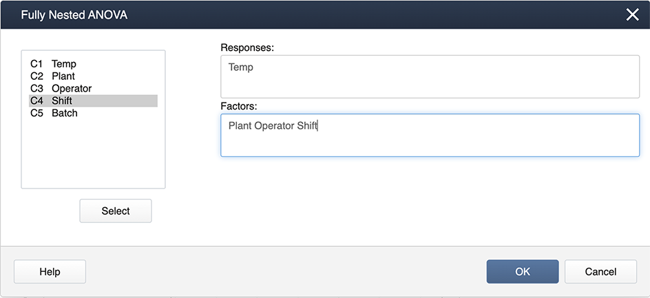
The output you get is very comprehensive and includes the variance components expressed as percentages.
Nested ANOVA: Temp versus Plant, Operator, Shift
Analysis of Variance for Temp
| Source | DF | SS | MS | F | P |
|---|---|---|---|---|---|
| Plant | 3 | 731.5156 | 243.8385 | 5.854 | 0.011 |
| Operator | 12 | 499.8125 | 41.6510 | 1.303 | 0.248 |
| Shift | 48 | 1534.9167 | 31.9774 | 2.578 | 0.000 |
| Error | 128 | 1588.0000 | 12.4062 | ||
| Total | 191 | 4354.2448 |
Variance Components
| Source | Var Comp. | # of Total | StDev |
|---|---|---|---|
| Plant | 4.212 | 17.59 | 2.052 |
| Operator | 0.806 | 3.37 | 0.898 |
| Shift | 6.524 | 27.24 | 2.554 |
| Error | 12.406 | 51.80 | 3.522 |
| Total | 23.948 | 4.894 |
Expected Mean Squares
| 1 | Plant | 1.00(4) + 3.00(3) + 12.00(2) + 48.00(1) |
|---|---|---|
| 2 | Operator | 1.00(4) + 3.00(3) + 12.00(2) |
| 3 | Shift | 1.00(4) + 3.00(3) |
| 4 | Error | 1.00(4) |
First, load and attach the quality data in R.
setwd("~/path-to-folder/")
quality_data<-read.table("quality_data.txt",header=T,sep ="\t")
attach(quality_data)
We then fit the fully nested random effects model. There are no fixed effects, so we display only the LRT table for the random effects.
library(lme4,lmerTest)
lm_rand = lmer(Temp ~ (1 | Plant) + (1 | Plant:Operator) + (1 | Plant:(Operator:Shift)))
ranova(lm_rand)
ANOVA-like table for random-effects: Single term deletions
Model:
Temp ~ (1 | Plant) + (1 | Plant:Operator) + (1 | Plant:(Operator:Shift))
npar logLik AIC LRT Df Pr(>Chisq)
5 -548.59 1107.2
(1 | Plant) 4 -551.03 1110.1 4.8755 1 0.02724 *
(1 | Plant:Operator) 4 -548.77 1105.5 0.3530 1 0.55240
(1 | Plant:(Operator:Shift)) 4 -557.36 1122.7 17.5317 1 2.826e-05 ***
---
Signif. codes: 0 ‘***’ 0.001 ‘**’ 0.01 ‘*’ 0.05 ‘.’ 0.1 ‘ ’ 1
NTo examine the variance components further we print the estimates.
vc = VarCorr(lm_rand, parm="theta_", oldNames = FALSE)
print(vc,comp=c("Variance"))
Groups Name Variance Plant:(Operator:Shift) (Intercept) 6.52371 Plant:Operator (Intercept) 0.80614 Plant (Intercept) 4.21227 Residual 12.40626
We can compute the variance percentages manually.
terms = data.frame(vc)$grp
vars = data.frame(vc)$vcov
tot_var = sum(vars)
percent_var = (vars/tot_var)*100
data.frame(cbind(terms,vars,percent_var))
terms vars percent_var
1 Plant:(Operator:Shift) 6.52370980810034 27.2407289699471
2 Plant:Operator 0.806136528703026 3.36614400964098
3 Plant 4.21226520994903 17.5889452947895
4 Residual 12.4062556768176 51.8041817256224
Note R does not produce the EMS coefficients, so if those are of interest another software may be useful.
6.5 - Introduction to Mixed Models
6.5 - Introduction to Mixed ModelsTreatment designs can be comprised of both fixed and random effects. When we have this situation, the treatment design is referred to as a mixed model. Mixed models are by far the most commonly encountered treatment designs. The three possible situations we now have are often referred to as Model I (fixed effects only), Model II (random effects only), and Model III (mixed) ANOVAs. When designating the effects of a mixed model as fixed or random, the following rule will be useful.
Below are the ANOVA layouts of two basic mixed models with 2-factors.
Factorial
In the simplest case of a balanced mixed model in a factorial design, we may have two factors, A and B, in which factor A is a fixed effect and factor B is a random effect. The statistical model is similar to what we have seen before:
\(y_{ijk} = \mu + \alpha_i + \beta_j + (\alpha\beta)_{ij} + \epsilon_{ijk}\) where \(i=1,2,\dots, a\), \(j=1,2,\dots, b\) and \(k=1,2, \dots, n\).
Here, \(\sum_{i} \alpha_i = 0, \) \(\beta_j \sim \mathcal{N}\left(0, \sigma^2_{\beta}\right), \) \((\alpha\beta)_{i,j} \sim N(0,\sigma^2_{\alpha\beta}) \) and \(\epsilon_{ijk} \sim \mathcal{N}\left(0, \sigma^2\right)\). Also, \(\beta_j, (\alpha\beta)_{ij}\) and \(\epsilon_{ij}\) are pairwise independent.
In this case, we have the following ANOVA:
Source | DF | EMS |
|---|---|---|
A | (a-1) | \(\sigma^2+n\sigma_{\alpha\beta}^{2}+nb\frac{\sum\alpha_{i}^{2}}{a-1}\) |
B | (b-1) | \(\sigma^2+n\sigma_{\alpha\beta}^{2}+na\sigma_{\beta}^{2}\) |
A \(\times\) B | (a-1)(b-1) | \(\sigma^2+n\sigma_{\alpha\beta}^{2}\) |
Error | ab(n-1) | \(\sigma^2\) |
Total | abn-1 |
The F-tests are set up based on the EMS column above and we can see that we have to use different denominators in testing significance for the various sources in the ANOVA table:
Source | EMS | F |
|---|---|---|
A | \(\sigma^2+n\sigma_{\alpha\beta}^{2}+nb\frac{\sum\alpha_{i}^{2}}{a-1}\) | MSA / MSAB |
B | \(\sigma^2+n\sigma_{\alpha\beta}^{2}+na\sigma_{\beta}^{2}\) | MSB / MSAB |
A × B | \(\sigma^2+n\sigma_{\alpha\beta}^{2}\) | MSAB / MSE |
Error | \(\sigma^2\) | |
Total |
As a reminder, the null hypothesis for a fixed effect is that the \(\alpha_i\)'s are equal, whereas the null hypothesis for the random effect is that the \(\sigma_{\beta}^{2}\) is equal to zero.
It is important to mention that the mixed model presented here is known as the “unrestricted model”, which is the model utilized in SAS as well. However, there is another “restricted” version of this model which is used in our course text. In practice, the most important difference between these models is how the F-stat for the random effect is calculated. More specifically, for the unrestricted model here it is MSB/MSAB, whereas for the restricted model, it is MSB/MSE. You can read more about the differences between these models in STAT 503 Section 13.3.
Nested
In the case of a balanced nested treatment design, where A is a fixed effect and B(A) is a random effect, the statistical model would be:
\(y_{ijk} = \mu + \alpha_i + \beta_{j(i)} + \epsilon_{ijk}\) where \(i=1,2,\dots, a\), \(j=1,2,\dots, b\) and \(k=1,2, \dots, n\).
Here, \(\sum_{i} \alpha_i = 0\), \(\beta_{j(i)} \sim \mathcal{N}\left(0, \sigma^2_{\beta(\alpha)}\right)\) and \(\epsilon_{ijk} \sim \mathcal{N}\left(0, \sigma^2\right)\).
We have the following ANOVA for this model:
Source | DF | EMS |
|---|---|---|
A | (a-1) | \(\sigma_{\epsilon}^{2}+n\sigma_{\beta(\alpha)}^{2}+bn\frac{\sum\alpha_{i}^{2}}{a-1}\) |
B(A) | a(b-1) | \(\sigma_{\epsilon}^{2}+n\sigma_{\beta(\alpha)}^{2}\) |
Error | ab(n-1) | \(\sigma_{\epsilon}^{2}\) |
Total | abn-1 |
Here is the same table with the F-statistics added. Note that the denominators for the F-test are different.
Source | EMS | F |
|---|---|---|
A | \(\sigma_{\epsilon}^{2}+n\sigma_{\beta(\alpha)}^{2}+bn\frac{\sum\alpha_{i}^{2}}{a-1}\) | MSA / MSB(A) |
B(A) | \(\sigma_{\epsilon}^{2}+n\sigma_{\beta(\alpha)}^{2}\) | MSB(A) / MSE |
Error | \(\sigma_{\epsilon}^{2}\) | |
Total |
F-Calculation Facts
As can be seen from the examples above (and in the previous sections), when significance testing in random or mixed models the denominator of the F-statistic is no longer always the MSE value and has to be aptly chosen. Recall that the F-statistic for testing the significance of a given effect is the ratio with the numerator equal to the MS value of the effect, and the denominator is also an MS value of an effect included in the ANOVA model. Furthermore, it can be said the F-statistic has a non-central distribution when \(H_a\) is true and a central F-distribution when \(H_0\) is true.
When \(H_a\) is true, the non-centrality parameter of the non-central F-distribution depends on the type of effect (fixed vs random) and equals \(\sum_{i=1}^T {\alpha_{i}^2}\) for a fixed effect and \(\sigma_{trt}^2\) for a random effect. Here \(\alpha_i=\mu_i-\mu\), where \(\mu_i\) is the \(i^{th}\) level of the fixed effect for \((i=1,2,...,T)\), \(\mu\) is the overall mean, and \(\sigma_{trt}^2\) is the variance component associated with the random effect. Also, the MS under true \(H_a\) equals to MS under true \(H_0\) plus non-centrality parameter, so that
F-statistic = \(\dfrac{\text{MS when \(H_0\) is true + non-centrality parameter}}{\text{MS when \(H_0\) is true}}\).
The above identity can be used to identify the correct denominator (also called the error term) with the aid of EMS expressions displayed in the ANOVA table. This can be summarized by the following rule.
6.6 - Mixed Model: School Example
6.6 - Mixed Model: School ExampleConsider the experimental setting in which the investigators are interested in comparing the classroom self-ratings of teachers. They created a tool that can be used to self-rate the classrooms. The investigators are interested in comparing the Eastern vs. Western US regions, and the type of school (Public vs. Private). Investigators chose 2 teachers randomly from each combination and each teacher submits scores from 2 classes that they teach.
You can download the data at Schools Data.
If we carefully consider the information in the setup, we see that the US region makes sense as a fixed effect, and so does the type of school. However, the investigators are probably not interested in testing for significant differences among individual teachers they recruited for the study, but more realistically they would be interested in how much variation there is among teachers (a random effect).
For this example, we can use a mixed model in which we model teacher as a random effect nested within the factorial fixed treatment combinations of Region and School type.
Using Technology
In SAS we would set up the ANOVA as:
proc mixed data=school covtest method=type3;
class Region SchoolType Teacher Class;
model sr_score = Region SchoolType Region*SchoolType;
random Teacher(Region*SchoolType);
store out_school;
run;
In SAS proc mixed, we see that the fixed effects appear in the model statement, and the nested random effect appears in the random statement.
We get the following partial output:
| Type 3 Analysis of Variance | ||||||||
|---|---|---|---|---|---|---|---|---|
| Source | DF | Sum of Squares | Mean Square | Expected Mean Square | Error Term | Error DF | F Value | Pr > F |
| Region | 1 | 564.062500 | 564.062500 | Var(Residual) + 2 Var(Teach(Region*School)) + Q(Region,Region*SchoolType) | MS(Teach(Region*School)) | 4 | 24.07 | 0.0080 |
| SchoolType | 1 | 76.562500 | 76.562500 | Var(Residual) + 2 Var(Teach(Region*School)) + Q(SchoolType,Region*SchoolType) | MS(Teach(Region*School)) | 4 | 3.27 | 0.1450 |
| Region*SchoolType | 1 | 264.062500 | 264.062500 | Var(Residual) + 2 Var(Teach(Region*School)) + Q(Region*SchoolType) | MS(Teach(Region*School)) | 4 | 11.27 | 0.0284 |
| Teach(Region*School) | 4 | 93.750000 | 23.437500 | Var(Residual) + 2 Var(Teach(Region*School)) | MS(Residual) | 8 | 5.00 | 0.0257 |
| Residual | 8 | 37.500000 | 4.687500 | Var(Residual) | . | . | . | . |
The results for hypothesis tests for the fixed effects appear as:
| Type 3 Tests of Fixed Effects | ||||
|---|---|---|---|---|
| Effect | Num DF | Den DF | F Value | Pr > F |
| Region | 1 | 4 | 24.07 | 0.0080 |
| SchoolType | 1 | 4 | 3.27 | 0.1450 |
| Region*SchoolType | 1 | 4 | 11.27 | 0.0284 |
Given that the Region*SchoolType interaction is significant, the PLM procedure along with the lsmeans statement can be used to generate the Tukey mean comparisons and produce the groupings chart and the plots to identify what means differ significantly.
ods graphics on;
proc plm restore=out_school;
lsmeans Region*SchoolType / adjust=tukey plot=meanplot cl lines;
run;
| Region*SchoolType Least Squares Means | |||||||||
|---|---|---|---|---|---|---|---|---|---|
| Region | SchoolType | Estimate | Standard Error | DF | t Value | Pr > |t| | Alpha | Lower | Upper |
| EastUS | Private | 85.7500 | 2.4206 | 4 | 35.42 | <.0001 | 0.05 | 79.0293 | 92.4707 |
| EastUS | Public | 73.2500 | 2.4206 | 4 | 30.26 | <.0001 | 0.05 | 66.5293 | 79.9707 |
| WestUS | Private | 89.5000 | 2.4206 | 4 | 36.97 | <.0001 | 0.05 | 82.7793 | 96.2207 |
| WestUS | Public | 93.2500 | 2.4206 | 4 | 38.52 | <.0001 | 0.05 | 86.5293 | 99.9707 |

| Differences of Region*SchoolType Least Squares Means Adjustment for Multiple Comparisons: Tukey |
||||||||||||||
|---|---|---|---|---|---|---|---|---|---|---|---|---|---|---|
| Region | SchoolType | _Region | _SchoolType | Estimate | Standard Error | DF | t Value | Pr > |t| | Adj P | Alpha | Lower | Upper | Adj Lower | Adj Upper |
| EastUS | Private | EastUS | Public | 12.5000 | 3.4233 | 4 | 3.65 | 0.0217 | 0.0703 | 0.05 | 2.9955 | 22.0045 | -1.4356 | 26.4356 |
| EastUS | Private | WestUS | Private | -3.7500 | 3.4233 | 4 | -1.10 | 0.3349 | 0.7109 | 0.05 | -13.2545 | 5.7545 | -17.6856 | 10.1856 |
| EastUS | Private | WestUS | Public | -7.5000 | 3.4233 | 4 | -2.19 | 0.0936 | 0.2677 | 0.05 | -17.0045 | 2.0045 | -21.4356 | 6.4356 |
| EastUS | Public | WestUS | Private | -16.2500 | 3.4233 | 4 | -4.75 | 0.0090 | 0.0301 | 0.05 | -25.7545 | -6.7455 | -30.1856 | -2.3144 |
| EastUS | Public | WestUS | Public | -20.0000 | 3.4233 | 4 | -5.84 | 0.0043 | 0.0146 | 0.05 | -29.5045 | -10.4955 | -33.9356 | -6.0644 |
| WestUS | Private | WestUS | Public | -3.7500 | 3.4233 | 4 | -1.10 | 0.3349 | 0.7109 | 0.05 | -13.2545 | 5.7545 | -17.6856 | 10.1856 |
From the results, it is clear that the mean self-rating scores are highest for the public school in the west region. The difference mean scores for schools in the west region are significantly different from the mean scores for public schools in the east region.
The covtest option produces the results needed to test the significance of the random effect, Teach(Region*SchoolType) in terms of the following null and alternative hypothesis:
\(H_0: \sigma_{teacher}^2=0 \ \text{vs.} H_a: \sigma_{teacher}^2\ > 0\)
However, as the following display shows, covtest option uses the Wald Z-test, which is based on the z-score of the sample statistic and hence is appropriate only for large samples - specifically when the number of random effect levels is sufficiently large. Otherwise, this test may not be reliable.
| Covariance Parameter Estimates | ||||
|---|---|---|---|---|
| Cov Parm | Estimate | Standard Error |
Z Value | Pr Z |
| Teach(Region*School) | 9.3750 | 8.3689 | 1.12 | 0.2626 |
| Residual | 4.6875 | 2.3438 | 2.00 | 0.0228 |
Therefore, in this case, as the number of teachers employed is few, Wald's test may not be valid. It is more appropriate to use the ANOVA F-test for Teacher(Region*SchoolType). Note that the results from the ANOVA table suggest that the effects of the teacher within the region and school type are significant (Pr > F = 0.0257), whereas the results based on Wald's test suggest otherwise (since the p-value is 0.2626).
In Minitab, specifying the mixed model is a little different.
In Stat > ANOVA > General Linear Model > Fit General Linear Model
we complete the dialog box:
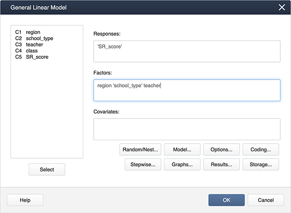
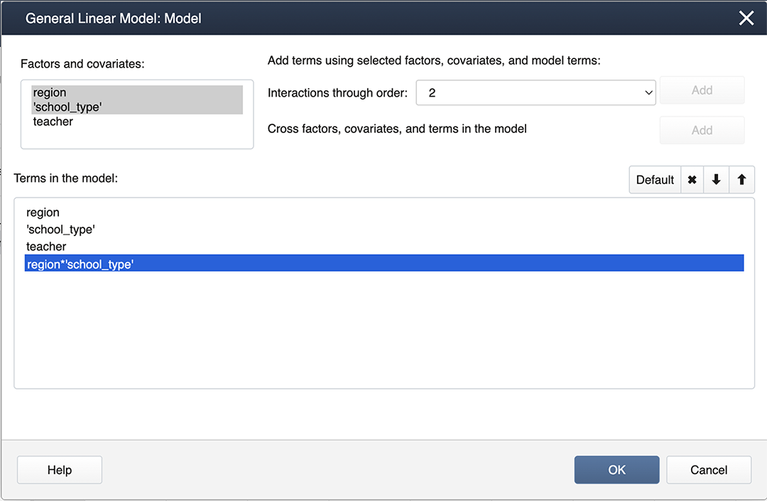
We can create interaction terms under Model… by selecting “region” and “school_type” and clicking Add.
Finally, we create nested terms and effects are random under Random/Nest…:
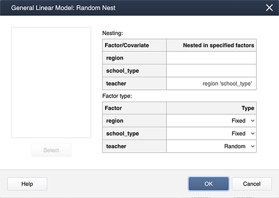
Minitab Output for the mixed model:
Factor Information
| Factor | Type | Levels | Values |
|---|---|---|---|
| region | Fixed | 2 | EastUS, WestUS |
| school_type | Fixed | 2 | Private, Public |
| teacher(region school_type) | Random | 8 | 1(EastUS,Private), 2(EastUS,Private,) 1(EastUS,Public), 2(EastUS, Public), 1(WestUS, Private), 2(WestUS, Private), 1(WestUS,Public), 2(WestUS,Public) |
Analysis of Variance
| Source | DF | Seq SS | Adj SS | Adj MS | F-Value | P-Value |
|---|---|---|---|---|---|---|
| region | 1 | 564.06 | 564.06 | 564.06 | 24.07 | 0.008 |
| school_type | 1 | 76.56 | 76.56 | 76.56 | 3.27 | 0.145 |
| region*school_type | 1 | 264.06 | 264.06 | 264.06 | 11.27 | 0.028 |
| teacher(region schoo_type) | 4 | 93.75 | 93.75 | 23.44 | 5.00 | 0.026 |
| Error | 8 | 37.50 | 37.50 | 4.69 | ||
| Total | 15 | 1035.94 |
Model Summary
| S | R-sq | R-sq(adj) | R-sq(pred) |
|---|---|---|---|
| 2.16506 | 96.38% | 93.21% | 85.52% |
Minitab’s results are in agreement with SAS Proc Mixed.
First, load and attach the schools data in R.
setwd("~/path-to-folder/")
schools_data<-read.table("schools_data.txt",header=T,sep ="\t")
attach(schools_data)
We then fit the mixed effects model and display the ANOVA table for the fixed effects and the LRT for the random effect.
library(lme4,lmerTest)
lm_rand<-lmer(SR_score ~ region + school_type + region:school_type + (1 | teacher:(region:school_type)))
anova(lm_rand)
Type III Analysis of Variance Table with Satterthwaite's method
                             Sum Sq Mean Sq NumDF DenDF F value Pr(>F)
region 112.812 112.812 1 4 24.0667 0.008011 **
school_type 15.312 15.312 1 4 3.2667 0.144986
region:school_type 52.812 52.812 1 4 11.2667 0.028395 *
---
Signif. codes: 0 ‘***’ 0.001 ‘**’ 0.01 ‘*’ 0.05 ‘.’ 0.1 ‘ ’ 1
ranova(lm_rand)
ANOVA-like table for random-effects: Single term deletions
Model:
SR_score ~ region + school_type + (1 | teacher:(region:school_type)) + region:school_type
npar logLik AIC LRT Df Pr(>Chisq)
6 -32.288 76.576
(1 | teacher:(region:school_type)) 5 -34.153 78.306 3.7298 1 0.05345 .
---
Signif. codes: 0 ‘***’ 0.001 ‘**’ 0.01 ‘*’ 0.05 ‘.’ 0.1 ‘ ’ 1
We can also examine the variance estimates and their 95% CIs.
vc = VarCorr(lm_rand)
                    print(vc,comp=c("Variance"))
Groups Name Variance teacher:(region:school_type) (Intercept) 9.3750 Residual 4.6875
ci_sig = confint(lm_rand, parm="theta_", oldNames = FALSE)
                    ci_sig2 = ci_sig^2
                    row.names(ci_sig2) = sapply(row.names(ci_sig2),function(x){gsub("sd_","var_",x)},USE.NAMES=FALSE)
                    row.names(ci_sig2)[length(row.names(ci_sig2))] = "sigma2"
                    ci_sig2
                                                2.5 %   97.5 %
var_(Intercept)|teacher:(region:school_type) 0.000000 16.62054
sigma2                                       2.017642 14.61089
Notice, the results of the LRT as well as the CIs suggest the random effect is not significant (different from the results of the F-test in SAS). However, the region and school type interaction is significant so we produce a Tukey pairwise analysis.
ls_means(lm_rand, "region:school_type", pairwise = TRUE)
lsmeans = emmeans::emmeans(lm_rand, pairwise~region:school_type, adjust="tukey")
ci = confint(lsmeans)
ci$contrasts
 contrast                        estimate   SE df lower.CL upper.CL
 EastUS Private - WestUS Private    -3.75 3.42  4   -17.69    10.19
 EastUS Private - EastUS Public     12.50 3.42  4    -1.44    26.44
 EastUS Private - WestUS Public     -7.50 3.42  4   -21.44     6.44
 WestUS Private - EastUS Public     16.25 3.42  4     2.31    30.19
 WestUS Private - WestUS Public     -3.75 3.42  4   -17.69    10.19
 EastUS Public - WestUS Public     -20.00 3.42  4   -33.94    -6.06
6.7 - Complexity Happens
6.7 - Complexity HappensFrom what we have discussed so far we see that even for the simplest multi-factor studies (i.e. those involving only two factors) there are many possibilities of treatment designs; each factor is either fixed or random as well as either crossed or nested.
For any of these possibilities, we can carry out the hypothesis tests using the EMS expressions to identify the correct denominator for the relevant F-statistics. The possible EMS expressions are summarized in the following tables.
| Crossed | ||||
|---|---|---|---|---|
| Source | d.f. | A fixed, B fixed | A fixed, B random | A random, B random |
| A | a-1 | \(\sigma^2+nb\frac{\sum\alpha_{i}^{2}}{a-1}\) | \(\sigma^2+n\sigma_{\alpha\beta}^2+nb\frac{\sum\alpha_{i}^{2}}{a-1}\) | \(\sigma^2 + nb\sigma_{\alpha}^2+n\sigma_{\alpha\beta}^2\) |
| B | b-1 | \(\sigma^2+na\frac{\sum\beta_{j}^{2}}{b-1}\) | \(\sigma^2 + n\sigma_{\alpha\beta}^2+ na\sigma_{\beta}^2\) | \(\sigma^2 + na\sigma_{\beta}^2+n\sigma_{\alpha\beta}^2\) |
| A×B | (a-1)(b-1) | \(\sigma^2+n\frac{\sum\sum(\alpha\beta)_{ij}^{2}}{(a-1)(b-1)}\) | \(\sigma^2 + n\sigma_{\alpha\beta}^2\) | \(\sigma^2 + n\sigma_{\alpha\beta}^2\) |
| Error | ab(n-1) | \(\sigma^2\) | \(\sigma^2\) | \(\sigma^2\) |
| Nested | ||||
|---|---|---|---|---|
| Source | d.f. | A fixed, B fixed | A fixed, B random | A random, B random |
| A | a-1 | \(\sigma^2+bn\frac{\sum\alpha_{i}^{2}}{a-1}\) | \(\sigma^2+bn\frac{\sum\alpha_{i}^{2}}{a-1}+n\sigma_{\beta(\alpha)}^2\) | \(\sigma^2 + bn\sigma_{\alpha}^2+n\sigma_{\beta(\alpha)}^2\) |
| B(A) | a(b-1) | \(\sigma^2+n\frac{\sum\sum\beta_{j(i)}^{2}}{a(b-1)}\) | \(\sigma^2 + n\sigma_{\beta(\alpha)}^2\) | \(\sigma^2 + n\sigma_{\beta(\alpha)}^2\) |
| Error | ab(n-1) | \(\sigma^2\) | \(\sigma^2\) | \(\sigma^2\) |
6.8 - Try it!
6.8 - Try it!Exercise 1
Three teaching methods were to be compared to teach computer science in high schools. Nine different schools were chosen randomly, and each teaching method was assigned to 3 randomly chosen schools, so each school implemented only one teaching method. The response used to compare the 3 teaching methods was the average score for each high school.
    data Lesson6_ex1;
    input mtd school score semester $;
    datalines;
    1 1 68.11 Fall
    1 1 68.11 Fall
    1 1 68.21 Fall
    1 1 78.11 Spring
    1 1 78.11 Spring
    1 1 78.19 Spring
    1 2 59.21 Fall
    1 2 59.13 Fall
    1 2 59.11 Fall
    1 2 70.18 Spring
    1 2 70.62 Spring
    1 2 69.11 Spring
    1 3 64.11 Fall
    1 3 63.11 Fall
    1 3 63.24 Fall
    1 3 63.21 Spring
    1 3 64.11 Spring
    1 3 63.11 Spring
    2 1 84.11 Fall
    2 1 85.21 Fall
    2 1 85.15 Fall
    2 1 85.11 Spring
    2 1 83.11 Spring
    2 1 89.21 Spring
    2 2 93.11 Fall
    2 2 95.21 Fall
    2 2 96.11 Fall
    2 2 95.11 Spring
    2 2 97.27 Spring
    2 2 94.11 Spring
    2 3 90.11 Fall
    2 3 88.19 Fall
    2 3 89.21 Fall
    2 3 90.11 Spring
    2 3 90.11 Spring
    2 3 92.21 Spring
    3 1 74.2 Fall
    3 1 78.14 Fall
    3 1 74.12 Fall
    3 1 87.1 Spring
    3 1 88.2 Spring
    3 1 85.1 Spring
    3 2 74.1 Fall
    3 2 73.14 Fall
    3 2 76.21 Fall
    3 2 72.14 Spring
    3 2 76.21 Spring
    3 2 75.1 Spring
    3 3 80.12 Fall
    3 3 79.27 Fall
    3 3 81.15 Fall
    3 3 85.23 Spring
    3 3 86.14 Spring
    3 3 87.19 Spring
    ;
-
Using the information about the teaching method, school, and score only, the school administrators conducted a statistical analysis to determine if the teaching method had a significant impact on student scores. Perform a statistical analysis to confirm their conclusion.
-
If possible, perform any other additional statistical analyses.
-
To confirm their conclusion, a model with only the two factors, teaching method, and school was used, with school nested within the teaching method.
Input:
    data Lesson6_ex1;
    input mtd school score semester $;
    datalines;
    1 1 68.11 Fall
    1 1 68.11 Fall
    1 1 68.21 Fall
    1 1 78.11 Spring
    1 1 78.11 Spring
    1 1 78.19 Spring
    1 2 59.21 Fall
    1 2 59.13 Fall
    1 2 59.11 Fall
    1 2 70.18 Spring
    1 2 70.62 Spring
    1 2 69.11 Spring
    1 3 64.11 Fall
    1 3 63.11 Fall
    1 3 63.24 Fall
    1 3 63.21 Spring
    1 3 64.11 Spring
    1 3 63.11 Spring
    2 1 84.11 Fall
    2 1 85.21 Fall
    2 1 85.15 Fall
    2 1 85.11 Spring
    2 1 83.11 Spring
    2 1 89.21 Spring
    2 2 93.11 Fall
    2 2 95.21 Fall
    2 2 96.11 Fall
    2 2 95.11 Spring
    2 2 97.27 Spring
    2 2 94.11 Spring
    2 3 90.11 Fall
    2 3 88.19 Fall
    2 3 89.21 Fall
    2 3 90.11 Spring
    2 3 90.11 Spring
    2 3 92.21 Spring
    3 1 74.2 Fall
    3 1 78.14 Fall
    3 1 74.12 Fall
    3 1 87.1 Spring
    3 1 88.2 Spring
    3 1 85.1 Spring
    3 2 74.1 Fall
    3 2 73.14 Fall
    3 2 76.21 Fall
    3 2 72.14 Spring
    3 2 76.21 Spring
    3 2 75.1 Spring
    3 3 80.12 Fall
    3 3 79.27 Fall
    3 3 81.15 Fall
    3 3 85.23 Spring
    3 3 86.14 Spring
    3 3 87.19 Spring
    ;


proc mixed data=lesson6_ex1 method=type3;
class mtd school;
model score = mtd;
random school(mtd);
store results1;
run;

proc plm restore=results1;
lsmeans mtd / adjust=tukey plot=meanplot cl lines;
run;
Partial outputs:
Type 3 Analysis of Variance
Type 3 Analysis of Variance Source DF Sum of Squares Mean Square Expected Mean Square Error Term Error DF F Value Pr > F mtd 2 4811.400959 2405.700480 Var(Residual) + 6 Var(school(mtd)) + Q(mtd) MS(school(mtd)) 6 16.50 0.0036 school(mtd) 6 875.059744 145.843291 Var(Residual) + 6 Var(school(mtd)) MS(Residual) 45 10.13 <.0001 Residual 45 647.972350 14.399386 Var(Residual) . . . . The p-value of 0.0036 indicates that the scores vary significantly among the 3 teaching methods, confirming the school administrators’ conclusion. As the teaching method was significant, the Tukey procedure was conducted to determine the significantly different pairs among the 3 teaching methods. The results of the Tukey procedure shown below indicate that the mean scores of teaching methods 2 and 3 are not statistically significant and that the teaching method 1 mean score is statistically lower than the mean scores of the other two.


- Using the additional code shown below, an ANOVA was conducted including semester also as a fixed effect.
proc mixed data=lesson6_ex1 method=type3;
class mtd school semester ;
model score = mtd semester mtd*semester;
random  school(mtd) semester*school(mtd);
store results2;
run;

proc plm restore= results2;
lsmeans mtd semester / adjust=tukey plot=meanplot cl lines;
run;
Type 3 Analysis of Variance
Type 3 Analysis of Variance Source DF Sum of Squares Mean Square Expected Mean Square Error Term Error DF F Value Pr > F mtd 2 4811.400959 2405.700480 Var(Residual) + 3 Var(school*semester(mtd)) + 6 Var(school(mtd)) + Q(mtd,mtd*semester) MS(school(mtd)) 6 16.50 0.0036 semester 1 286.166224 286.166224 Var(Residual) + 3 Var(school*semester(mtd)) + Q(semester,mtd*semester) MS(school*semester(mtd)) 6 8.34 0.0278 mtd*semester 2 85.703404 42.851702 Var(Residual) + 3 Var(school*semester(mtd)) + Q(mtd*semester) MS(school*semester(mtd)) 6 1.25 0.3520 school(mtd) 6 875.059744 145.843291 Var(Residual) + 3 Var(school*semester(mtd)) + 6 Var(school(mtd)) MS(school*semester(mtd)) 6 4.25 0.0508 school*semester(mtd) 6 205.848456 34.308076 Var(Residual) + 3 Var(school*semester(mtd)) MS(Residual) 36 17.58 <.0001 Residual 36 70.254267 1.951507 Var(Residual) . . . . The p-values indicate both the main effects of the method and semester are statistically significant, but their interaction is not and can be removed from the model. The Tukey procedure indicates that the significances of paired comparisons for the teaching method remain the same as in the previous model. Between the two semesters, the scores are statistically higher in the spring compared to the fall.
Note! The output writes semester*school(mtd) as school*semester(mtd) due to SAS arranging effects in alphabetical order.semester Least Squares Means semester Estimate Standard Error DF t Value Pr > |t| Alpha Lower Upper Fall 76.6370 1.8265 6 41.96 <.0001 0.05 72.1677 81.1063 Spring 81.2411 1.8265 6 44.48 <.0001 0.05 76.7718 85.7104
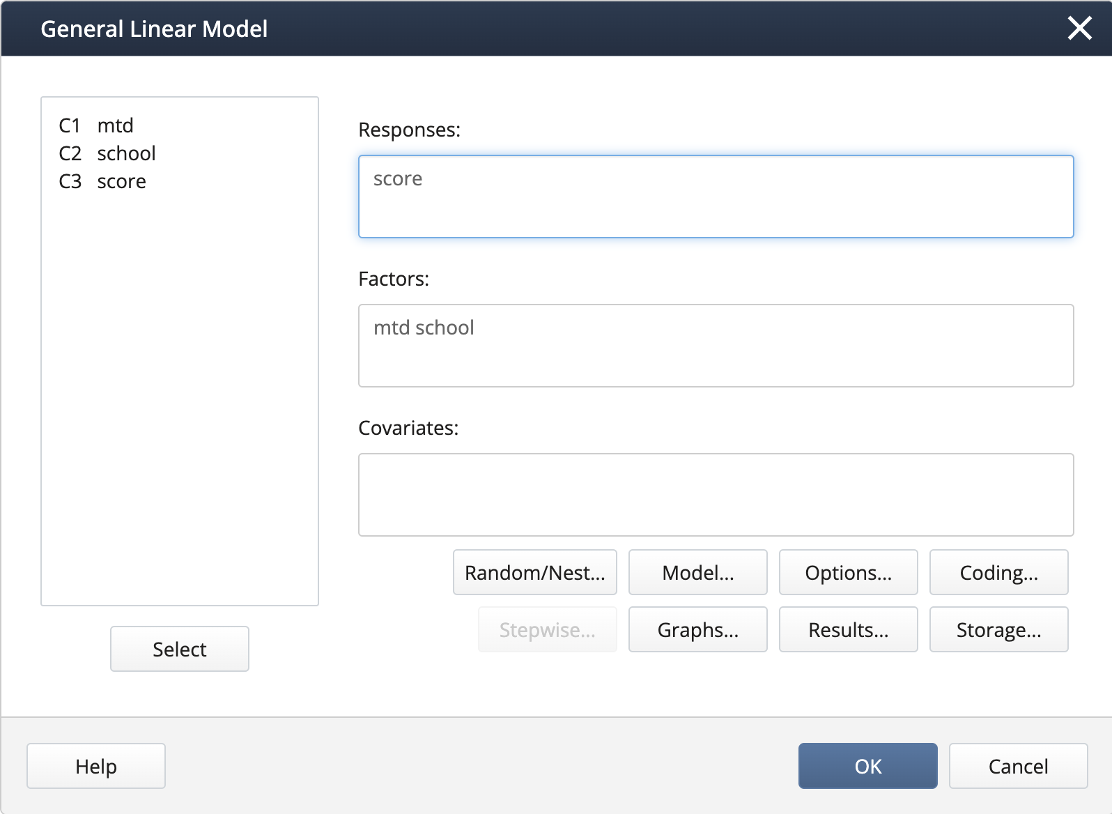
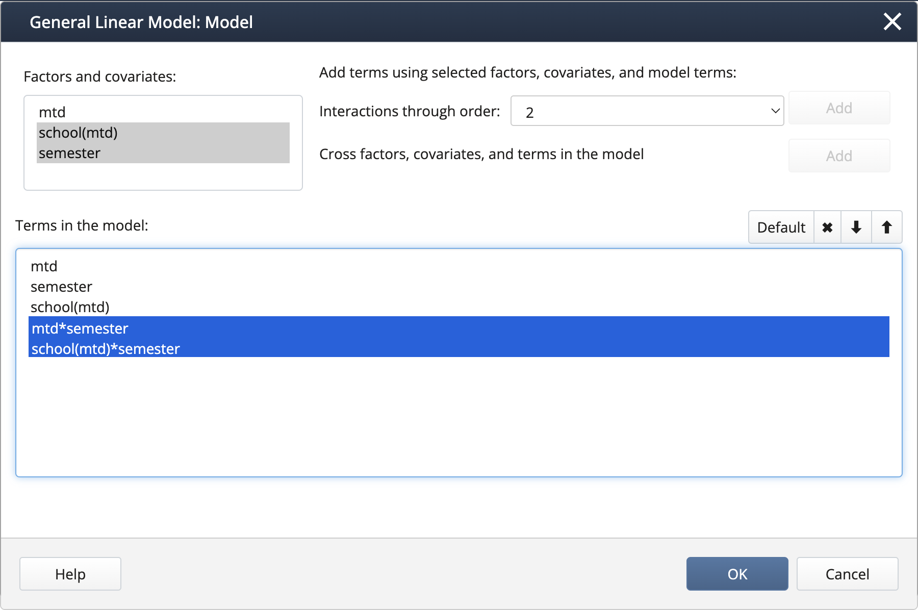
- In Stat > ANOVA > General Linear Model > Fit General Linear Model we complete the dialog box:
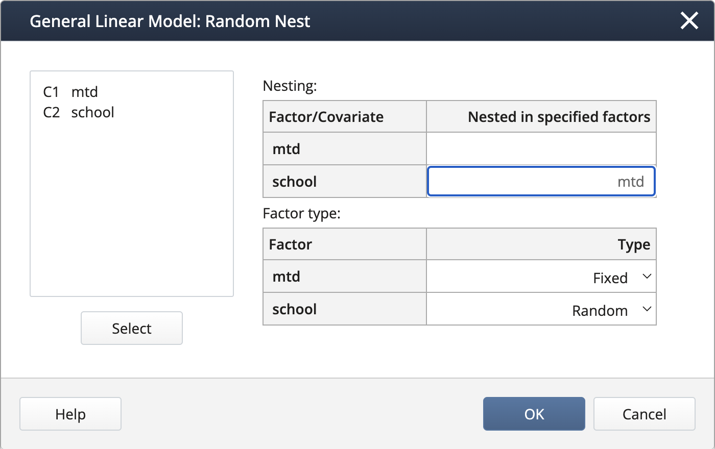
We create the nested term and specify the random effects under Random/Nest…:
Output:
Analysis of Variance
Source DF Adj SS Adj MS F-Value P-Value mtd 2 4811.4 2405.70 16.50 0.004 school(mtd) 6 875.1 145.84 10.13 0.000 Error 45 648.0 14.40 Total 53 6334.4 The p-value of 0.004 indicates that mtd is statistically significant. This implies that the mean score from all 3 teaching methods is not the same, confirming the school administrators’ claim. Note that in Minitab General Linear Model, the Tukey procedure or any other paired comparisons are not available.
-
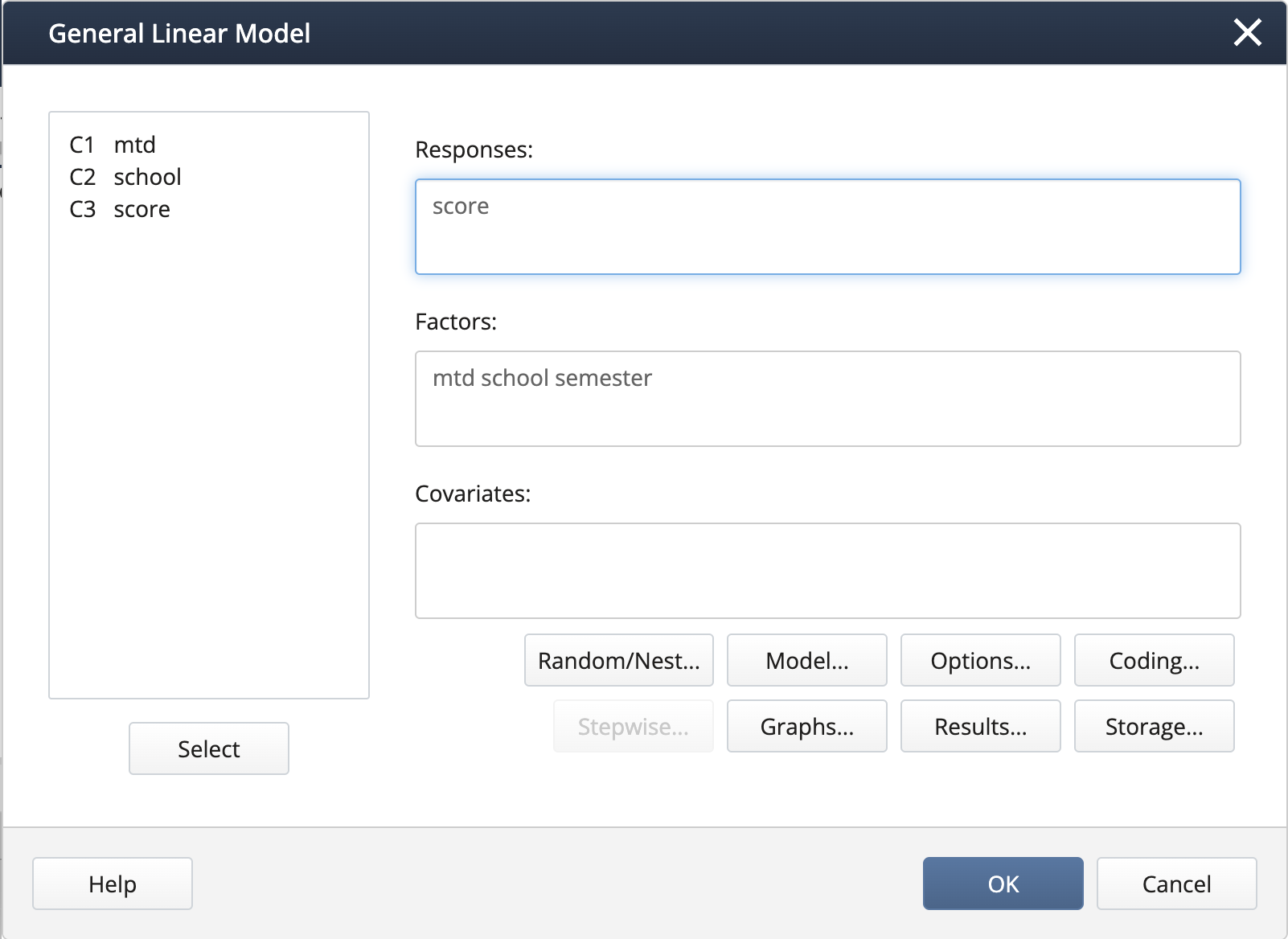
In Stat > ANOVA > General Linear Model > Fit General Linear Model we complete the dialog box:
We create the nested term and specify the random effects under Random/Nest…:
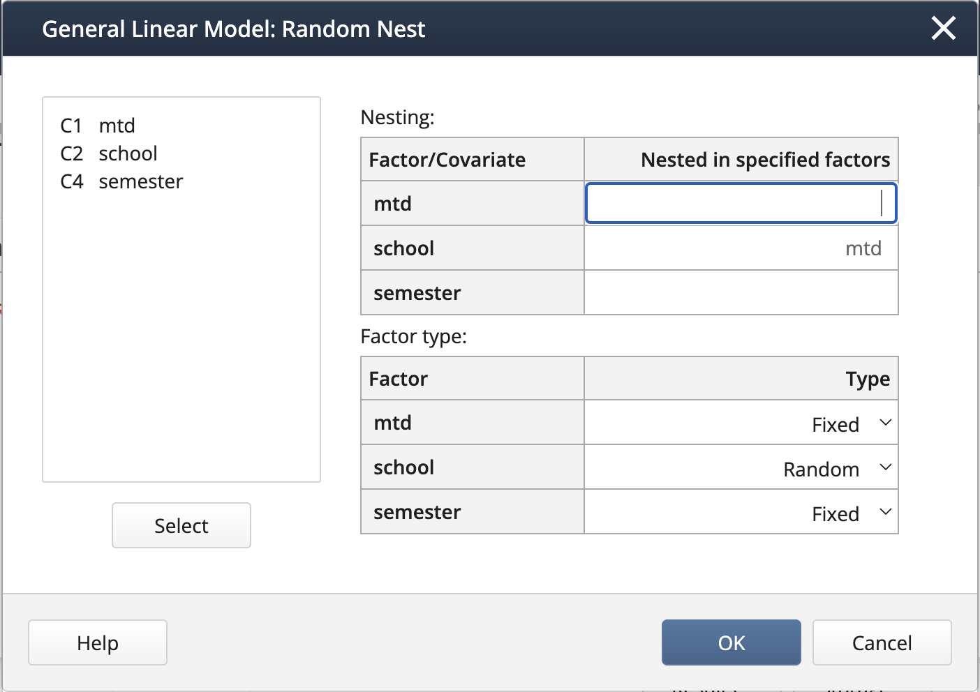
We can create interaction terms under Model… by selecting “mtd” and “semester” and clicking Add, then repeating for “school(mtd)” and “semester”.
Output:
Analysis of Variance
Source DF Adj SS Adj MS F-Value P-Value mtd 2 4811.40 2405.70 16.50 0.004 semester 1 286.17 286.17 8.34 0.028 school(mtd) 6 875.06 145.84 4.25 0.051 mtd*semester 2 85.70 42.85 1.25 0.352 school(mtd)*semester 6 205.85 34.31 17.58 0.000 Error 36 70.25 1.95 Total 53 6334.43 The p-values indicate that both main effects mtd and semester are statistically significant, but not their interaction.
Exercise 2
| Type 3 Analysis of Variance | ||||||
|---|---|---|---|---|---|---|
| Source | DF | Sum of Squares | Mean Square | Expected Mean Square | F Value | Pr > F |
| Residual | 2 | 4811.400959 | 2405.700480 | Var(Residual) + 6 Var(A*B) + Q(A) | 11.38 | 0.0224 |
| 2 | 29.274959 | 14.637480 | Var(Residual) + 6 Var(A*B) + 18 Var(B) | 1.02 | 0.3700 | |
| 4 | 845.784785 | 211.446196 | Var(Residual)+ 6 Var(A*B) | 14.68 | <.0001 | |
| 45 | 647.972350 | 14.399386 | Var(Residual) | . | . | |
Use the ANOVA table above to answer the following.
- Name the fixed and random effects.
- Complete the Source column of the ANOVA table above.
- How many observations are included in this study?
- How many replicates are there?
- Write the model equation.
- Write the hypotheses that can be tested with the expression for the appropriate F statistic.
-
Name the fixed and random effects.
Fixed: A with 3 levels. In the EMS column, Q(A) reveals that A is fixed and the df indicates that it has 3 levels. Note that any factor that has a quadratic form associated with it is fixed and Q(A) is the quadratic form associated with A. This actually equals \(\sum_{i=1}^3\alpha_i^2\) where \(i = 1,2, 3\) are the treatment effects and is non-zero if the treatment means are significantly different.
Random: B is random as indicated by the presence of Var(B). The effect of factor B is studied by sampling 3 cases (see df value for B). A*B is random as any effect involving a random factor is random. The residual is also random as indicated by the presence of the Var(residual) in the EMS column.
-
Complete the Source column of the ANOVA table above.
Use the EMS column and start from the bottom row. The bottom-most has only Var(residual) and therefore the effect on the corresponding Source is residual. The next row up has Var(A*B) in the additional term indicating that the corresponding source is A*B, etc.
Type 3 Analysis of Variance Source DF Sum of Squares Mean Square Expected Mean Square F Value Pr > F A 2 4811.400959 2405.700480 Var(Residual) + 6 Var(A*B) + Q(A) 11.38 0.0224 B 2 29.274959 14.637480 Var(Residual) + 6 Var(A*B) + 18 Var(B) 1.02 0.3700 A*B 4 845.784785 211.446196 Var(Residual)+ 6 Var(A*B) 14.68 <.0001 Residual 45 647.972350 14.399386 Var(Residual) . . -
How many observations are included in this study?
N-1 = 2 + 2 +4 + 45 = 53 so N = 54.
-
How many full replicates are there?
Let r = number of replicates. Then N = number of levels of A * number of levels of B * r = 3 * 3 * r. Therefore, \(9 \times r = 54\) which gives \(r=6\).
-
Write the model equation.
\(y_{ijk}=\mu+\alpha_i+\beta_j+(\alpha\beta)_{ij}+\epsilon_{ijk},\text{ }i,j=1,2,3\text{, and }k = 1,2,\dots,6\)
-
Write the hypotheses that can be tested with the F-statistic information.
Effect A
Hypotheses
\(H_0\colon\alpha_i=0 \text{ for all } i\) vs. \(H_a\colon\alpha_i \neq 0\), for at least one \(i=1,2,3\)
Note that \(\sum_{i=1}^3\alpha_i^2\) is the non-centrality parameter of the F statistics if \(H_a\) is true.F-statistic
\(\dfrac{2405.700480}{211.446196}=11.377\) with 2 and 4 degrees of freedom
Effect B
Hypotheses
\(H_0\colon\sigma_\beta^2=0\) vs. \(H_a\colon \sigma_\beta^2 > 0\)
F-statistic
\(\dfrac{14.63480}{211.446196}=0.0692\) with 2 and 4 degrees of freedom
Note that SAS uses the unrestricted model (mentioned in Section 6.5) which results in MSAB as the denominator of the F-test (verified by looking at the EMS expressions).
Effect A*B
Hypotheses
\(H_0\colon\sigma_{\alpha\beta}^2=0\) vs. \(H_a\colon\sigma_{\alpha\beta}^2> 0\)
F-statistic
\(\dfrac{211.446196}{14.399386}=14.685\) with 4 and 45 degrees of freedom
6.9 - Lesson 6 Summary
6.9 - Lesson 6 SummaryRandom effects of an ANOVA model represent measurements arising from a larger population. In other words, the levels or groups of the random effect that are observed can be considered as a sample from an original population. Random effects can also be subject effects. Consequently, in public health, a random effect is sometimes referred to as the subject-specific effect.
As all the levels of a random effect have the same mean, its significance is measured in terms of the variance with \(H_0\colon \sigma_{\tau}^2=0 \ \text{vs.}\ H_a\colon\sigma_{\tau}^2\gt0\). Note also that any interaction effect involving at least one random effect is also a random effect. Due to the added variability incurred by each random effect, the variance of the response now will have several components which are called variance components. In the most basic case only one single factor and no fixed effects, this compound variance of the response will be \(\sigma_{Y}^2=\sigma_{\tau}^2+\sigma_{\epsilon}^2\), where \(\sigma_{\tau}^2\) is the variance component associated with the random factor. The intra-class correlation (ICC), defined in terms of the variance components, is a useful indicator of the high or low variability within groups (or subjects).
Mixed models introduced in section 6.5 include both fixed and random effects. Throughout the lesson, we learned how EMS quantities can be used to determine the correct F-test to test the hypotheses associated with the effects. EMS quantities can be thought of as the population counterparts of the mean sums of squares (MS) which are computable for each source in the ANOVA table.