6.4 - Fully Nested Random Effects Model: Quality Control Example
6.4 - Fully Nested Random Effects Model: Quality Control ExampleThe temperature of a process in a manufacturing industry is critical to quality control. The researchers want to characterize the sources of this variability. They choose 4 plants, 4 operators within each plant, look at 4 shifts for each operator, and then measure temperature for each of the three batches used in production.
Collected data was read into SAS and proc mixed procedure was used to obtain the ANOVA model.
data fullnest;
input Temp Plant Operator Shift Batch;
datalines;
477   1   1   1   1
472   1   1   1   2
481   1   1   1   3
478   1   1   2   1
475   1   1   2   2
474   1   1   2   3
472   1   1   3   1
475   1   1   3   2
468   1   1   3   3
482   1   1   4   1
477   1   1   4   2
474   1   1   4   3
471   1   2   1   1
474   1   2   1   2
470   1   2   1   3
479   1   2   2   1
482   1   2   2   2
477   1   2   2   3
470   1   2   3   1
477   1   2   3   2
483   1   2   3   3
480   1   2   4   1
473   1   2   4   2
478   1   2   4   3
475   1   3   1   1
472   1   3   1   2
470   1   3   1   3
460   1   3   2   1
469   1   3   2   2
472   1   3   2   3
477   1   3   3   1
483   1   3   3   2
475   1   3   3   3
476   1   3   4   1
480   1   3   4   2
471   1   3   4   3
465   1   4   1   1
464   1   4   1   2
471   1   4   1   3
477   1   4   2   1
475   1   4   2   2
471   1   4   2   3
481   1   4   3   1
477   1   4   3   2
475   1   4   3   3
470   1   4   4   1
475   1   4   4   2
474   1   4   4   3
484   2   1   1   1
477   2   1   1   2
481   2   1   1   3
477   2   1   2   1
482   2   1   2   2
481   2   1   2   3
479   2   1   3   1
477   2   1   3   2
482   2   1   3   3
477   2   1   4   1
470   2   1   4   2
479   2   1   4   3
472   2   2   1   1
475   2   2   1   2
475   2   2   1   3
472   2   2   2   1
475   2   2   2   2
470   2   2   2   3
472   2   2   3   1
477   2   2   3   2
475   2   2   3   3
482   2   2   4   1
477   2   2   4   2
483   2   2   4   3
485   2   3   1   1
481   2   3   1   2
477   2   3   1   3
482   2   3   2   1
483   2   3   2   2
485   2   3   2   3
477   2   3   3   1
476   2   3   3   2
481   2   3   3   3
479   2   3   4   1
476   2   3   4   2
485   2   3   4   3
477   2   4   1   1
475   2   4   1   2
476   2   4   1   3
476   2   4   2   1
471   2   4   2   2
472   2   4   2   3
475   2   4   3   1
475   2   4   3   2
472   2   4   3   3
481   2   4   4   1
470   2   4   4   2
472   2   4   4   3
475   3   1   1   1
470   3   1   1   2
469   3   1   1   3
477   3   1   2   1
471   3   1   2   2
474   3   1   2   3
469   3   1   3   1
473   3   1   3   2
468   3   1   3   3
477   3   1   4   1
475   3   1   4   2
473   3   1   4   3
470   3   2   1   1
466   3   2   1   2
468   3   2   1   3
471   3   2   2   1
473   3   2   2   2
476   3   2   2   3
478   3   2   3   1
480   3   2   3   2
474   3   2   3   3
477   3   2   4   1
471   3   2   4   2
469   3   2   4   3
466   3   3   1   1
465   3   3   1   2
471   3   3   1   3
473   3   3   2   1
475   3   3   2   2
478   3   3   2   3
471   3   3   3   1
469   3   3   3   2
471   3   3   3   3
475   3   3   4   1
477   3   3   4   2
472   3   3   4   3
469   3   4   1   1
471   3   4   1   2
468   3   4   1   3
473   3   4   2   1
475   3   4   2   2
473   3   4   2   3
477   3   4   3   1
470   3   4   3   2
469   3   4   3   3
463   3   4   4   1
471   3   4   4   2
469   3   4   4   3
484   4   1   1   1
477   4   1   1   2
480   4   1   1   3
476   4   1   2   1
475   4   1   2   2
474   4   1   2   3
475   4   1   3   1
470   4   1   3   2
469   4   1   3   3
481   4   1   4   1
476   4   1   4   2
472   4   1   4   3
469   4   2   1   1
475   4   2   1   2
479   4   2   1   3
482   4   2   2   1
483   4   2   2   2
479   4   2   2   3
477   4   2   3   1
479   4   2   3   2
475   4   2   3   3
472   4   2   4   1
476   4   2   4   2
479   4   2   4   3
470   4   3   1   1
481   4   3   1   2
481   4   3   1   3
475   4   3   2   1
470   4   3   2   2
475   4   3   2   3
469   4   3   3   1
477   4   3   3   2
482   4   3   3   3
485   4   3   4   1
479   4   3   4   2
474   4   3   4   3
469   4   4   1   1
473   4   4   1   2
475   4   4   1   3
477   4   4   2   1
473   4   4   2   2
471   4   4   2   3
470   4   4   3   1
468   4   4   3   2
474   4   4   3   3
483   4   4   4   1
477   4   4   4   2
476   4   4   4   3
;
proc mixed data=fullnest covtest method=type3;
class Plant Operator Shift Batch;
model temp=;
random plant operator(plant) shift(plant operator) ;
run;
In the SAS code, notice that there are no terms on the right-hand side of the model statement. This is because SAS uses the model statement to specify fixed effects only. The random statement is used to specify the random effects. The proc mixed procedure will perform the fully nested random effects model as specified above, and produces the following output:
| Type 3 Analysis of Variance | ||||||||
|---|---|---|---|---|---|---|---|---|
| Source | DF | Sum of Squares | Mean Square | Expected Mean Square | Error Term | Error DF | F Value | Pr > F |
| Plant | 3 | 731.515625 | 243.838542 | Var(Residual) + 3 Var(Shift(Plant*Operato)) + 12 Var(Operator(Plant)) + 48 Var(Plant) | MS(Operator(Plant)) | 12 | 5.85 | 0.0106 |
| Operator(Plant) | 12 | 499.812500 | 41.651042 | Var(Residual) + 3 Var(Shift(Plant*Operato)) + 12 Var(Operator(Plant)) | MS(Shift(Plant*Operato)) | 48 | 1.30 | 0.2483 |
| Shift(Plant*Operato) | 48 | 1534.916667 | 31.977431 | Var(Residual) + 3 Var(Shift(Plant*Operato)) | MS(Residual) | 128 | 2.58 | <.0001 |
| Residual | 128 | 1588.000000 | 12.406250 | Var(Residual) | . | . | . | . |
| Covariance Parameter Estimates | ||||
|---|---|---|---|---|
| Cov Parm | Estimate | Standard Error |
Z Value | Pr Z |
| Plant | 4.2122 | 4.1629 | 1.01 | 0.3116 |
| Operator(Plant) | 0.8061 | 1.5178 | 0.53 | 0.5953 |
| Shift(Plant*Operato) | 6.5237 | 2.2364 | 2.92 | 0.0035 |
| Residual | 12.4063 | 1.5508 | 8.00 | <.0001 |
The largest (and significant) variance components are: (1) the shift within a plant \(\times\) operator combination and (2) the batch-to-batch variation within the shift (the residual).
Note that the Covariance Parameter Estimates here are in fact the variance components. SAS does not express the variance components as percentages in this procedure, but by summing the variance components for all sources to serve as the denominator, each source can be expressed as a percentage.
Because this type of model is so commonly employed, SAS also offers two other procedures to obtain the variance components results: proc varcomp (which stands for variance components) and proc nested.
The equivalent code for these procedures is as follows:
The proc varcomp:
proc varcomp data=fullnest;
class  Plant Operator Shift Batch;
model temp= plant operator(plant) shift(plant operator);
run;
Note that the model statement for proc varcomp differs from the mixed procedure in that proc varcomp assumes that the factors listed in the model statement are random effects.
Partial Output:
| MIVQUE(0) Estimates | |
|---|---|
| Variance Component | Temp |
| Var(Plant) | 4.21224 |
| Var(Operator(Plant)) | 0.80613 |
| Var(Shift(Plant*Operato)) | 6.52373 |
| Var(Error) | 12.40625 |
Note that, even in this procedure we will have to use the sum for a total and calculate the percentages ourselves. On the other hand, the proc nested procedure will provide the full output including the percentages:
proc nested data=fullnest;
class plant operator shift;
var temp;
run;
Partial Output:
| Nested Random Effects Analysis of Variance for Variable Temp | ||||||||
|---|---|---|---|---|---|---|---|---|
| Variance Source | DF | Sum of Squares | F Value | Pr > F | Error Term | Mean Square | Variance Component | Percent of Total |
| Total | 191 | 4354.244792 | 22.797093 | 23.948351 | 100.0000 | |||
| Plant | 3 | 731.515625 | 5.85 | 0.0106 | Operator | 243.838542 | 4.212240 | 17.5889 |
| Operator | 12 | 499.812500 | 1.30 | 0.2483 | Shift | 41.651042 | 0.806134 | 3.3661 |
| Shift | 48 | 1534.916667 | 2.58 | <.0001 | Error | 31.977431 | 6.523727 | 27.2408 |
| Error | 128 | 1588.000000 | 12.406250 | 12.406250 | 51.8042 | |||
Calculation of the Variance Components
From the SAS output, we get the EMS coefficients. We can use those to compute the estimated variance components.
| Source | MS | EMS | Variance Components | % Variation |
|---|---|---|---|---|
| Plant | 243.84 | \(\sigma_{\epsilon}^{2}+3\sigma_{\gamma}^{2}+12\sigma_{\beta}^{2}+48\sigma_{\alpha}^{2}\) | 4.21 | 17.58 |
| Operator(Plant) | 41.65 | \(\sigma_{\epsilon}^{2}+3\sigma_{\gamma}^{2}+12\sigma_{\beta}^{2}\) | 0.806 | 3.37 |
| Shift(Plant × Operator) | 31.98 | \(\sigma_{\epsilon}^{2}+3\sigma_{\gamma}^{2}\) | 6.52 | 27.24 |
| Residual | 12.41 | \(\sigma_{\epsilon}^{2}\) | 12.41 | 51.80 |
| Total | 23.95 |
One can show that MS is an unbiased estimator for EMS (using the properties of Method of Moments estimates). With that, we can algebraically solve for each variance component. Start at the bottom of the table and work up the hierarchy.
First of all, the estimated variance component for the Residuals is given:
\(\mathbf{12.41} = \hat{\sigma}_{\text{error}}^{2}\) = \(\hat{\sigma}_{\epsilon}^{2}\)
Then we can use this information and subtract it from the Shift(Plant \(\times\) Operator) MS to get:
\(\begin{align}31.98 &= \hat{\sigma}_{\epsilon}^{2}+3\hat{\sigma}_{\gamma \text{ or Shift(Plant*Operator)}}^{2} \\[10pt] \hat{\sigma}_{\gamma}^{2}&=\frac{31.98-12.41}{3}=\mathbf{6.52}\end{align}\)
Similarly, we use what we know for Error and Shift(Plant \(\times\) Operator) and subtract it from the Operator(Plant) MS to get:
\(\begin{align}41.65&=\hat{\sigma}_{\epsilon}^{2}+3\hat{\sigma}_{\gamma}^{2} +12\hat{\sigma}_{\beta \text{ or Operator(Plant)}}^{2}\\[10pt] &=31.98+12\hat{\sigma}_{\beta}^{2}\\[10pt] \hat{\sigma}_{\beta}^{2}&=\frac{41.65-31.98}{12}\\[10pt] &=\mathbf{0.806}\end{align}\)
And finally, we use what we know for Error and Shift(Plant \(\times\) Operator) and Operator(Plant), subtract it from the Plant MS to get:
\(\begin{align}243.84&=\hat{\sigma}_{\epsilon}^{2}+3\hat{\sigma}_{\gamma}^{2} +12\hat{\sigma}_{\beta}^{2}+48\hat{\sigma}_{\alpha \text{ or Plant}}^{2}\\[10pt] &=41.65+48\hat{\sigma}_{\alpha}^{2}\\[10pt] \hat{\sigma}_{\alpha}^{2}&=\frac{243.84-41.65}{48}\\[10pt] &=\mathbf{4.21}\end{align}\)
Our total = 12.41 + 6.52 + 0.806 + 4.21 = 23.95
Then, dividing each variance component by the total gives the % values shown in the output from SAS proc nested.
Minitab has a separate program just for this type of analysis for our example (Quality Data ), under:
Stat > ANOVA > Fully Nested ANOVA
and you specify the model in the boxes provided:
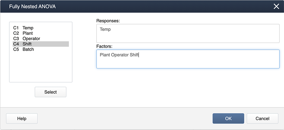
The output you get is very comprehensive and includes the variance components expressed as percentages.
Nested ANOVA: Temp versus Plant, Operator, Shift
Analysis of Variance for Temp
| Source | DF | SS | MS | F | P |
|---|---|---|---|---|---|
| Plant | 3 | 731.5156 | 243.8385 | 5.854 | 0.011 |
| Operator | 12 | 499.8125 | 41.6510 | 1.303 | 0.248 |
| Shift | 48 | 1534.9167 | 31.9774 | 2.578 | 0.000 |
| Error | 128 | 1588.0000 | 12.4062 | ||
| Total | 191 | 4354.2448 |
Variance Components
| Source | Var Comp. | # of Total | StDev |
|---|---|---|---|
| Plant | 4.212 | 17.59 | 2.052 |
| Operator | 0.806 | 3.37 | 0.898 |
| Shift | 6.524 | 27.24 | 2.554 |
| Error | 12.406 | 51.80 | 3.522 |
| Total | 23.948 | 4.894 |
Expected Mean Squares
| 1 | Plant | 1.00(4) + 3.00(3) + 12.00(2) + 48.00(1) |
|---|---|---|
| 2 | Operator | 1.00(4) + 3.00(3) + 12.00(2) |
| 3 | Shift | 1.00(4) + 3.00(3) |
| 4 | Error | 1.00(4) |
First, load and attach the quality data in R.
setwd("~/path-to-folder/")
quality_data<-read.table("quality_data.txt",header=T,sep ="\t")
attach(quality_data)
We then fit the fully nested random effects model. There are no fixed effects, so we display only the LRT table for the random effects.
library(lme4,lmerTest)
lm_rand = lmer(Temp ~ (1 | Plant) + (1 | Plant:Operator) + (1 | Plant:(Operator:Shift)))
ranova(lm_rand)
ANOVA-like table for random-effects: Single term deletions

Model:
Temp ~ (1 | Plant) + (1 | Plant:Operator) + (1 | Plant:(Operator:Shift))
                             npar  logLik    AIC     LRT Df Pr(>Chisq)
                                5 -548.59 1107.2
(1 | Plant)                     4 -551.03 1110.1  4.8755  1    0.02724 *
(1 | Plant:Operator)            4 -548.77 1105.5  0.3530  1    0.55240
(1 | Plant:(Operator:Shift))    4 -557.36 1122.7 17.5317  1  2.826e-05 ***
---
Signif. codes:  0 ‘***’ 0.001 ‘**’ 0.01 ‘*’ 0.05 ‘.’ 0.1 ‘ ’ 1
NTo examine the variance components further we print the estimates.
vc = VarCorr(lm_rand, parm="theta_", oldNames = FALSE)
print(vc,comp=c("Variance"))
 Groups                 Name        Variance
 Plant:(Operator:Shift) (Intercept)  6.52371
 Plant:Operator         (Intercept)  0.80614
 Plant                  (Intercept)  4.21227
 Residual                           12.40626
We can compute the variance percentages manually.
terms = data.frame(vc)$grp
vars = data.frame(vc)$vcov
tot_var = sum(vars)
percent_var = (vars/tot_var)*100
data.frame(cbind(terms,vars,percent_var))
                   terms              vars      percent_var
1 Plant:(Operator:Shift)  6.52370980810034 27.2407289699471
2         Plant:Operator 0.806136528703026 3.36614400964098
3                  Plant  4.21226520994903 17.5889452947895
4               Residual  12.4062556768176 51.8041817256224
Note R does not produce the EMS coefficients, so if those are of interest another software may be useful.