6.6 - Mixed Model: School Example
6.6 - Mixed Model: School ExampleConsider the experimental setting in which the investigators are interested in comparing the classroom self-ratings of teachers. They created a tool that can be used to self-rate the classrooms. The investigators are interested in comparing the Eastern vs. Western US regions, and the type of school (Public vs. Private). Investigators chose 2 teachers randomly from each combination and each teacher submits scores from 2 classes that they teach.
You can download the data at Schools Data.
If we carefully consider the information in the setup, we see that the US region makes sense as a fixed effect, and so does the type of school. However, the investigators are probably not interested in testing for significant differences among individual teachers they recruited for the study, but more realistically they would be interested in how much variation there is among teachers (a random effect).
For this example, we can use a mixed model in which we model teacher as a random effect nested within the factorial fixed treatment combinations of Region and School type.
Using Technology
In SAS we would set up the ANOVA as:
proc mixed data=school covtest method=type3;
class Region SchoolType Teacher Class;
model sr_score = Region SchoolType Region*SchoolType;
random Teacher(Region*SchoolType);
store out_school;
run;
In SAS proc mixed, we see that the fixed effects appear in the model statement, and the nested random effect appears in the random statement.
We get the following partial output:
| Type 3 Analysis of Variance | ||||||||
|---|---|---|---|---|---|---|---|---|
| Source | DF | Sum of Squares | Mean Square | Expected Mean Square | Error Term | Error DF | F Value | Pr > F |
| Region | 1 | 564.062500 | 564.062500 | Var(Residual) + 2 Var(Teach(Region*School)) + Q(Region,Region*SchoolType) | MS(Teach(Region*School)) | 4 | 24.07 | 0.0080 |
| SchoolType | 1 | 76.562500 | 76.562500 | Var(Residual) + 2 Var(Teach(Region*School)) + Q(SchoolType,Region*SchoolType) | MS(Teach(Region*School)) | 4 | 3.27 | 0.1450 |
| Region*SchoolType | 1 | 264.062500 | 264.062500 | Var(Residual) + 2 Var(Teach(Region*School)) + Q(Region*SchoolType) | MS(Teach(Region*School)) | 4 | 11.27 | 0.0284 |
| Teach(Region*School) | 4 | 93.750000 | 23.437500 | Var(Residual) + 2 Var(Teach(Region*School)) | MS(Residual) | 8 | 5.00 | 0.0257 |
| Residual | 8 | 37.500000 | 4.687500 | Var(Residual) | . | . | . | . |
The results for hypothesis tests for the fixed effects appear as:
| Type 3 Tests of Fixed Effects | ||||
|---|---|---|---|---|
| Effect | Num DF | Den DF | F Value | Pr > F |
| Region | 1 | 4 | 24.07 | 0.0080 |
| SchoolType | 1 | 4 | 3.27 | 0.1450 |
| Region*SchoolType | 1 | 4 | 11.27 | 0.0284 |
Given that the Region*SchoolType interaction is significant, the PLM procedure along with the lsmeans statement can be used to generate the Tukey mean comparisons and produce the groupings chart and the plots to identify what means differ significantly.
ods graphics on;
proc plm restore=out_school;
lsmeans Region*SchoolType / adjust=tukey plot=meanplot cl  lines;
run;
| Region*SchoolType Least Squares Means | |||||||||
|---|---|---|---|---|---|---|---|---|---|
| Region | SchoolType | Estimate | Standard Error | DF | t Value | Pr > |t| | Alpha | Lower | Upper |
| EastUS | Private | 85.7500 | 2.4206 | 4 | 35.42 | <.0001 | 0.05 | 79.0293 | 92.4707 |
| EastUS | Public | 73.2500 | 2.4206 | 4 | 30.26 | <.0001 | 0.05 | 66.5293 | 79.9707 |
| WestUS | Private | 89.5000 | 2.4206 | 4 | 36.97 | <.0001 | 0.05 | 82.7793 | 96.2207 |
| WestUS | Public | 93.2500 | 2.4206 | 4 | 38.52 | <.0001 | 0.05 | 86.5293 | 99.9707 |

| Differences of Region*SchoolType Least Squares Means Adjustment for Multiple Comparisons: Tukey |
||||||||||||||
|---|---|---|---|---|---|---|---|---|---|---|---|---|---|---|
| Region | SchoolType | _Region | _SchoolType | Estimate | Standard Error | DF | t Value | Pr > |t| | Adj P | Alpha | Lower | Upper | Adj Lower | Adj Upper |
| EastUS | Private | EastUS | Public | 12.5000 | 3.4233 | 4 | 3.65 | 0.0217 | 0.0703 | 0.05 | 2.9955 | 22.0045 | -1.4356 | 26.4356 |
| EastUS | Private | WestUS | Private | -3.7500 | 3.4233 | 4 | -1.10 | 0.3349 | 0.7109 | 0.05 | -13.2545 | 5.7545 | -17.6856 | 10.1856 |
| EastUS | Private | WestUS | Public | -7.5000 | 3.4233 | 4 | -2.19 | 0.0936 | 0.2677 | 0.05 | -17.0045 | 2.0045 | -21.4356 | 6.4356 |
| EastUS | Public | WestUS | Private | -16.2500 | 3.4233 | 4 | -4.75 | 0.0090 | 0.0301 | 0.05 | -25.7545 | -6.7455 | -30.1856 | -2.3144 |
| EastUS | Public | WestUS | Public | -20.0000 | 3.4233 | 4 | -5.84 | 0.0043 | 0.0146 | 0.05 | -29.5045 | -10.4955 | -33.9356 | -6.0644 |
| WestUS | Private | WestUS | Public | -3.7500 | 3.4233 | 4 | -1.10 | 0.3349 | 0.7109 | 0.05 | -13.2545 | 5.7545 | -17.6856 | 10.1856 |
From the results, it is clear that the mean self-rating scores are highest for the public school in the west region. The difference mean scores for schools in the west region are significantly different from the mean scores for public schools in the east region.
The covtest option produces the results needed to test the significance of the random effect, Teach(Region*SchoolType) in terms of the following null and alternative hypothesis:
\(H_0: \sigma_{teacher}^2=0 \ \text{vs.} H_a: \sigma_{teacher}^2\ > 0\)
However, as the following display shows, covtest option uses the Wald Z-test, which is based on the z-score of the sample statistic and hence is appropriate only for large samples - specifically when the number of random effect levels is sufficiently large. Otherwise, this test may not be reliable.
| Covariance Parameter Estimates | ||||
|---|---|---|---|---|
| Cov Parm | Estimate | Standard Error |
Z Value | Pr Z |
| Teach(Region*School) | 9.3750 | 8.3689 | 1.12 | 0.2626 |
| Residual | 4.6875 | 2.3438 | 2.00 | 0.0228 |
Therefore, in this case, as the number of teachers employed is few, Wald's test may not be valid. It is more appropriate to use the ANOVA F-test for Teacher(Region*SchoolType). Note that the results from the ANOVA table suggest that the effects of the teacher within the region and school type are significant (Pr > F = 0.0257), whereas the results based on Wald's test suggest otherwise (since the p-value is 0.2626).
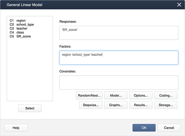
In Minitab, specifying the mixed model is a little different.
In Stat > ANOVA > General Linear Model > Fit General Linear Model
we complete the dialog box:
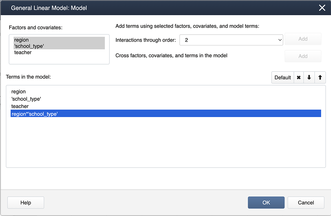
We can create interaction terms under Model… by selecting “region” and “school_type” and clicking Add.
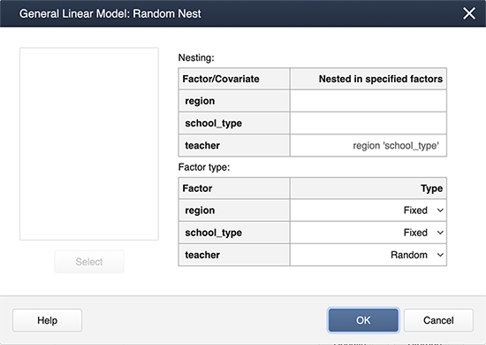
Finally, we create nested terms and effects are random under Random/Nest…:
Minitab Output for the mixed model:
Factor Information
| Factor | Type | Levels | Values |
|---|---|---|---|
| region | Fixed | 2 | EastUS, WestUS |
| school_type | Fixed | 2 | Private, Public |
| teacher(region school_type) | Random | 8 | 1(EastUS,Private), 2(EastUS,Private,) 1(EastUS,Public), 2(EastUS, Public), 1(WestUS, Private), 2(WestUS, Private), 1(WestUS,Public), 2(WestUS,Public) |
Analysis of Variance
| Source | DF | Seq SS | Adj SS | Adj MS | F-Value | P-Value |
|---|---|---|---|---|---|---|
| region | 1 | 564.06 | 564.06 | 564.06 | 24.07 | 0.008 |
| school_type | 1 | 76.56 | 76.56 | 76.56 | 3.27 | 0.145 |
| region*school_type | 1 | 264.06 | 264.06 | 264.06 | 11.27 | 0.028 |
| teacher(region schoo_type) | 4 | 93.75 | 93.75 | 23.44 | 5.00 | 0.026 |
| Error | 8 | 37.50 | 37.50 | 4.69 | ||
| Total | 15 | 1035.94 |
Model Summary
| S | R-sq | R-sq(adj) | R-sq(pred) |
|---|---|---|---|
| 2.16506 | 96.38% | 93.21% | 85.52% |
Minitab’s results are in agreement with SAS Proc Mixed.
First, load and attach the schools data in R.
setwd("~/path-to-folder/")
schools_data<-read.table("schools_data.txt",header=T,sep ="\t")
attach(schools_data)
We then fit the mixed effects model and display the ANOVA table for the fixed effects and the LRT for the random effect.
library(lme4,lmerTest)
lm_rand<-lmer(SR_score ~ region + school_type + region:school_type + (1 | teacher:(region:school_type)))
anova(lm_rand)
Type III Analysis of Variance Table with Satterthwaite's method
                    Sum Sq Mean Sq NumDF DenDF F value   Pr(>F)
region             112.812 112.812     1     4 24.0667 0.008011 **
school_type         15.312  15.312     1     4  3.2667 0.144986
region:school_type  52.812  52.812     1     4 11.2667 0.028395 *
---
Signif. codes:  0 ‘***’ 0.001 ‘**’ 0.01 ‘*’ 0.05 ‘.’ 0.1 ‘ ’ 1
ranova(lm_rand)
ANOVA-like table for random-effects: Single term deletions

Model:
SR_score ~ region + school_type + (1 | teacher:(region:school_type)) + region:school_type
                                   npar  logLik    AIC    LRT Df Pr(>Chisq)
                                      6 -32.288 76.576
(1 | teacher:(region:school_type))    5 -34.153 78.306 3.7298  1    0.05345 .
---
Signif. codes:  0 ‘***’ 0.001 ‘**’ 0.01 ‘*’ 0.05 ‘.’ 0.1 ‘ ’ 1
We can also examine the variance estimates and their 95% CIs.
vc = VarCorr(lm_rand)
print(vc,comp=c("Variance"))
 Groups                       Name        Variance
 teacher:(region:school_type) (Intercept) 9.3750
 Residual                                 4.6875
ci_sig = confint(lm_rand, parm="theta_", oldNames = FALSE)
ci_sig2 = ci_sig^2
row.names(ci_sig2) = sapply(row.names(ci_sig2),function(x){gsub("sd_","var_",x)},USE.NAMES=FALSE)
row.names(ci_sig2)[length(row.names(ci_sig2))] = "sigma2"
ci_sig2
                                                2.5 %   97.5 %
var_(Intercept)|teacher:(region:school_type) 0.000000 16.62054
sigma2                                       2.017642 14.61089
Notice, the results of the LRT as well as the CIs suggest the random effect is not significant (different from the results of the F-test in SAS). However, the region and school type interaction is significant so we produce a Tukey pairwise analysis.
ls_means(lm_rand, "region:school_type", pairwise = TRUE)
lsmeans = emmeans::emmeans(lm_rand, pairwise~region:school_type, adjust="tukey")
ci = confint(lsmeans)
ci$contrasts
 contrast                        estimate   SE df lower.CL upper.CL
 EastUS Private - WestUS Private    -3.75 3.42  4   -17.69    10.19
 EastUS Private - EastUS Public     12.50 3.42  4    -1.44    26.44
 EastUS Private - WestUS Public     -7.50 3.42  4   -21.44     6.44
 WestUS Private - EastUS Public     16.25 3.42  4     2.31    30.19
 WestUS Private - WestUS Public     -3.75 3.42  4   -17.69    10.19
 EastUS Public - WestUS Public     -20.00 3.42  4   -33.94    -6.06