7: Randomization Design Part I
7: Randomization Design Part IOverview
Introduction to Randomization Design
Previously in the course, we have referenced how experimental design drives the statistical model to be fitted. Recall in Lesson 5, we discussed the two components of the experimental design that accounts for two aspects of a study.
The first aspect, the treatment design component (addressed in Lessons 5 and 6) describes the treatment levels of interest, treatment type (fixed vs. random), and also the relationship of treatments with each other (crossed vs. nested).
In this lesson we will begin to learn about the second aspect, the randomization design. This component takes into account the treatment design aspects as well as the physical layout of the study setting including other influencing factors such as confounding (or blocking) variables.
In our discussions of treatment designs, we looked at experimental data in which there were multiple observations made at the treatment applications. We referred to these loosely as replicates. In this lesson, we will work formally with these multiple observations and how they are to be collected. This brings us to the right-hand side of the following schematic diagram, portraying the randomization design component.
Experimental Design
Treatment Design
How many factors are there?
How many levels of each factor are there?
If there is more than 1 factor, how are they related?
Crossed (Factorial): each level of factors occurs with all levels of other factors.
Nested: levels of a factor are unique to different levels of another factor.
Are factors fixed or random effects?
Are there any continuous covariates? (ANCOVA)
Randomization Design
What is the experimental unit?
An experimental unit is defined as that which receives a treatment, (e.g., plant, person, plot of ground, petri dish, etc.).
Is there more than one experimental unit? (Split Plot)
How are treatment levels assigned to experimental units?
Completely at random? CRD
Restriction or randomization?
One-dimension: RCBD
Two-dimension: Latin Square (LSD)
Are there sample units within experimental units? How many true replications are there?
Are there repeated measurements made on experimental units?
As can be seen in the diagram above, the treatment design addresses specific characteristics of the experimental factors under study. The randomization design addresses how the treatments are assigned to experimental units. Overall, the experimental design facilitates collecting data systematically as well as dictates the statistical model and the ANOVA-related calculations to be used in the analysis.
Objectives
- Understand the importance of randomization design, the second component of experimental design and how it impacts on our interpretation of results.
- Identify any blocking factors and the randomization design used in a study.
- Use statistical software to obtain the randomization design that assigns the treatment levels to the experimental units schematically.
- Gain experience in utilizing statistical software to analyze data obtained from a given experimental design.
7.1 - Experimental Unit and Replication
7.1 - Experimental Unit and Replication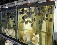
An experimental unit is an item (or physical entity) that receives the treatment. Identifying the experimental unit can be a trivial task in most experiments, but there can be exceptions.
For example...
Consider a situation where the effect of polluted stream water on fish lesions is to be studied. Two aquaria each with 50 fish are used for the study. The water treatment (polluted vs. control) is randomly assigned to each of the aquaria. After 30 days, the number of lesions was counted from randomly caught 10 fish from each aquarium. The treatment design is a single-factor design with 2 levels of water treatment, and a one-way ANOVA can be run on the data... but what is the experimental unit?Going back to our definition, the experimental unit is the entity that receives the treatment. In this case, we have applied a water treatment to each aquarium. The fish are not the experimental units. In order for individual fish to be experimental units, somehow the investigators would have to take one fish at a time and apply the treatment independently to each fish. This would be impractical from a logistics standpoint and was not done. Instead, the water treatment levels were applied to the entire aquarium, and so the experimental unit is an aquarium with 50 fish.
Now we can determine what constitutes a replication of the experiment. Each time the full set of treatment levels (2 levels in our example) is applied, we have a complete replication. Therefore in the experiment described there is only one replication; a situation often described as an un-replicated study.
The individual fish that were caught and counted for lesions are sampling units. Sampling units are the entities from which the observations are recorded. Traditionally, to obtain a correct ANOVA, mean values of the sampling units have to be computed for each experimental unit before the calculation of the treatment SS. Failure to recognize sampling units can result in a serious problem: pseudo-replication. Pseudo-replication results from treating each sampling unit as if it were an experimental unit and inflating the error degrees of freedom. By artificially increasing the error df, we reduce the MSE and produce a larger (incorrect) F-statistic.
7.2 - Completely Randomized Design (CRD)
7.2 - Completely Randomized Design (CRD)After identifying the experimental unit and the number of replications that will be used, the next step is to assign the treatments (i.e. factor levels or factor level combinations) to the experimental units.
In a completely randomized design (CRD), treatments are assigned to experimental units at random. This is typically done by listing the treatments and assigning a random number to each.
In the greenhouse experiment discussed in lesson 1, there was a single factor (fertilizer) with 4 levels (i.e. 4 treatments), six replications, and a total of 24 experimental units (potted plants). Suppose the image below is the greenhouse bench (viewed from above) that was used for the experiment.
We need to be able to randomly assign each of the treatment levels to 6 potted plants. To do this, we first assign numbers to the physical position of the pots on the bench.
Next, we randomly assign the 24 total treatments (4 treatment levels, replicated 6 times) to the potted plants. Examples of how this can be done using statistical software are found below.
Using Technology
To make the assignments in SAS we can utilize the SAS surveyselect procedure seen below.
proc surveyselect data=greenhouse out=trtassignment outrandom
method=srs
samprate=1;
run;
The output would be as below. In practice, it is recommended to specify a seed to ensure the results are reproducible.
| Obs | Fertilizer |
|---|---|
| 1 | F3 |
| 2 | F2 |
| 3 | Con |
| 4 | F2 |
| 5 | F3 |
| 6 | Con |
| 7 | F2 |
| 8 | F2 |
| 9 | F3 |
| 10 | F1 |
| 11 | F1 |
| 12 | F3 |
| 13 | F2 |
| 14 | F1 |
| 15 | F3 |
| 16 | F3 |
| 17 | F1 |
| 18 | Con |
| 19 | Con |
| 20 | F2 |
| 21 | Con |
| 22 | F1 |
| 23 | Con |
| 24 | F1 |
Next, select Calc > Sample from Columns, fill in the dialog box as seen below, and click OK.
This will result in a completely random assignment.
This assignment can then be used to apply the treatment levels appropriately to pots on the greenhouse bench.
To randomly assign treatment levels to each of our plants in R, we first create a vector containing all the possible treatments, then randomly sample from the vector to create the assignment.
trt_levels = c("F1","F2","F3","Control")
treatments = rep(trt_levels,6)

set.seed(1)
trt_assign = sample(treatments)
data.frame(trt_assign)
   trt_assign
1     Control
2          F3
3          F1
4          F2
5          F3
6          F2
7          F2
8          F2
9          F1
10    Control
11         F2
12         F2
13         F3
14         F3
15         F1
16         F3
17    Control
18         F1
19    Control
20    Control
21         F1
22         F1
23         F3
24    Control
7.3 - Randomized Complete Block Design (RCBD)
7.3 - Randomized Complete Block Design (RCBD)A CRD for the greenhouse experiment is reasonable, provided the positions on the bench are equivalent. In reality, this is rarely the case. For example, some micro-environmental variation can be expected due to the glass wall on one end, and the open walkway at the other end of the bench.
A powerful alternative to the CRD is to restrict the randomization process to form blocks. In a block design, general blocks are formed such that the experimental units are expected to be homogeneous within a block and heterogeneous between blocks. The number of experimental units within a block is called its block size.
In a randomized complete block design (RCBD), each block size is the same and is equal to the number of treatments (i.e. factor levels or factor level combinations). Furthermore, each treatment will be randomly assigned to exactly one experimental unit within every block. So if we think of the greenhouse example, in a RCBD we will have 6 blocks, each with block size of 4 (the number of fertilizer levels).
To establish an RCBD for this data, the assignments of fertilizer levels to the experimental units (the potted plants) have to be done within each block separately. Examples of how to do this using statistical software will be detailed in the section below.
It is important to mention that blocks are usually (but not always) treated as random effects as they typically represent the population of all possible blocks. In other words, the mean comparison among specific blocks is not of interest. However, the variation between blocks must be incorporated into the model. In a RCBD, the variation between blocks is partitioned out of the MSE of the CRD, resulting in a smaller MSE for testing hypotheses about the treatments.
The statistical model corresponding to the RCBD is similar to the two-factor studies with one observation per cell (i.e. we assume the two factors do not interact).
Here is Dr. Shumway stepping through this experimental design in the greenhouse.
We will consider the greenhouse experiment with one factor of interest (Fertilizer). We also have the identifications for the blocks. In this example, we consider Fertilizer as a fixed effect (as we are only interested in comparing the 4 fertilizers we chose for the study) and Block as a random effect.
Therefore the statistical model would be
\(Y_{ij} = \mu + \rho_i + \tau_j + \epsilon_{ij}\)
with \(i=1,2,\dots,6\) and \(j=1,2,3,4\). \(\rho_i\)s and \(\epsilon_{ij}\) are independent random variables such that \(\rho_i \sim \mathcal{N}\left(0, \sigma^2_{\rho}\right)\) and \(\epsilon_{ij}\sim \mathcal{N}\left(0, \sigma^2\right)\).
Using Technology
To obtain the block design in SAS, we can use the following code:
proc plan ordered ;
factors Block=6 Plant=4;
treatments Fertilizer=4 random;
output out=rcb block
cvals=('Block 1' 'Block 2' 'Block 3' 'Block 4' 'Block 5' 'Block 6');
run;
proc format;
value FertFmt
1 = "F1"
2 = "F2"
3 = "F3"
4 = "Con";
run;
proc print data=rcb;
format Fertilizer FertFmt.;
run;
The output we obtain would be as follows:
| Obs | Block | Plant | Fertilizer |
|---|---|---|---|
| 1 | Block 1 | 1 | F3 |
| 2 | Block 1 | 2 | F2 |
| 3 | Block 1 | 3 | Con |
| 4 | Block 1 | 4 | F1 |
| 5 | Block 2 | 1 | F1 |
| 6 | Block 2 | 2 | F3 |
| 7 | Block 2 | 3 | F2 |
| 8 | Block 2 | 4 | Con |
| 9 | Block 3 | 1 | F2 |
| 10 | Block 3 | 2 | Con |
| 11 | Block 3 | 3 | F3 |
| 12 | Block 3 | 4 | F1 |
| 13 | Block 4 | 1 | F2 |
| 14 | Block 4 | 2 | F3 |
| 15 | Block 4 | 3 | F1 |
| 16 | Block 4 | 4 | Con |
| 17 | Block 5 | 1 | F3 |
| 18 | Block 5 | 2 | F1 |
| 19 | Block 5 | 3 | Con |
| 20 | Block 5 | 4 | F2 |
| 21 | Block 6 | 1 | Con |
| 22 | Block 6 | 2 | F2 |
| 23 | Block 6 | 3 | F3 |
| 24 | Block 6 | 4 | F1 |
Once we collect the data for this experiment, we can use SAS to analyze the data and obtain the results.
Let us read the data into SAS and obtain the proc summary output.
data RCBD_oneway;
input block Fert $ Height;
datalines;
1      Control      19.5
2      Control      20.5
3      Control      21
4      Control      21
5      Control      21.5
6      Control      22.5
1      F1      25
2      F1      27.5
3      F1      28
4      F1      28.6
5      F1      30.5
6      F1      32
1      F2      22.5
2      F2      25.2
3      F2      26
4      F2      26.5
5      F2      27
6      F2      28
1      F3      27.5
2      F3      28
3      F3      29.2
4      F3      29.5
5      F3      30
6      F3      31
;
proc summary data=RCBD_oneway;
class block fert;
var height;
output out=output1 mean=mean stderr=se;
run;
proc print data=output1;
The proc summary output would be as follows. We see that the first line in the table with _TYPE_=0 identification is the estimated overall mean (i.e. \(\bar{y}_{\cdot\cdot}\)). The estimated treatment means (i.e. \(\bar{y}_{\cdot j}\)) are displayed with _TYPE_=1 identification and the estimated block means are displayed with _TYPE_=2 identification. Since we only have one observation per treatment within each block, we cannot estimate the standard error using the data.
| Obs | block | Fert | _TYPE_ | _FREQ_ | mean | se |
|---|---|---|---|---|---|---|
| 1 | . | 0 | 24 | 26.1667 | 0.75238 | |
| 2 | . | Control | 1 | 6 | 21.0000 | 0.40825 |
| 3 | . | F1 | 1 | 6 | 28.6000 | 0.99499 |
| 4 | . | F2 | 1 | 6 | 25.8667 | 0.77531 |
| 5 | . | F3 | 1 | 6 | 29.2000 | 0.52599 |
| 6 | 1 | 2 | 4 | 23.6250 | 1.71239 | |
| 7 | 2 | 2 | 4 | 25.3000 | 1.71221 | |
| 8 | 3 | 2 | 4 | 26.0500 | 1.80808 | |
| 9 | 4 | 2 | 4 | 26.4000 | 1.90657 | |
| 10 | 5 | 2 | 4 | 27.2500 | 2.06660 | |
| 11 | 6 | 2 | 4 | 28.3750 | 2.13478 | |
| 12 | 1 | Control | 3 | 1 | 19.5000 | . |
| 13 | 1 | F1 | 3 | 1 | 25.0000 | . |
| 14 | 1 | F2 | 3 | 1 | 22.5000 | . |
| 15 | 1 | F3 | 3 | 1 | 27.5000 | . |
| 16 | 2 | Control | 3 | 1 | 20.5000 | . |
| 17 | 2 | F1 | 3 | 1 | 27.5000 | . |
| 18 | 2 | F2 | 3 | 1 | 25.2000 | . |
| 19 | 2 | F3 | 3 | 1 | 28.0000 | . |
| 20 | 3 | Control | 3 | 1 | 21.0000 | . |
| 21 | 3 | F1 | 3 | 1 | 28.0000 | . |
| 22 | 3 | F2 | 3 | 1 | 26.0000 | . |
| 23 | 3 | F3 | 3 | 1 | 29.2000 | . |
| 24 | 4 | Control | 3 | 1 | 21.0000 | . |
| 25 | 4 | F1 | 3 | 1 | 28.6000 | . |
| 26 | 4 | F2 | 3 | 1 | 26.5000 | . |
| 27 | 4 | F3 | 3 | 1 | 29.5000 | . |
| 28 | 5 | Control | 3 | 1 | 21.5000 | . |
| 29 | 5 | F1 | 3 | 1 | 30.5000 | . |
| 30 | 5 | F2 | 3 | 1 | 27.0000 | . |
| 31 | 5 | F3 | 3 | 1 | 30.0000 | . |
| 32 | 6 | Control | 3 | 1 | 22.5000 | . |
| 33 | 6 | F1 | 3 | 1 | 32.0000 | . |
| 34 | 6 | F2 | 3 | 1 | 28.0000 | . |
| 35 | 6 | F3 | 3 | 1 | 31.0000 | . |
To run the model in SAS we can use the following code
/* RCBD */
proc mixed data=RCBD_oneway method=type3;
class block fert;
model height=fert;
random block;
run;
We obtain the ANOVA table below for the RCBD.
| Type 3 Analysis of Variance | ||||||||
|---|---|---|---|---|---|---|---|---|
| Source | DF | Sum of Squares | Mean Square | Expected Mean Square | Error Term | Error DF | F Value | Pr > F |
| Fert | 3 | 251.440000 | 83.813333 | Var(Residual) + Q(Fert) | MS(Residual) | 15 | 162.96 | <.0001 |
| block | 5 | 53.318333 | 10.663667 | Var(Residual) + 4 Var(block) | MS(Residual) | 15 | 20.73 | <.0001 |
| Residual | 15 | 7.715000 | 0.514333 | Var(Residual) | . | . | . | . |
For comparison, let us obtain the ANOVA table for the CRD for the same data. We use the following SAS commands:
/* CRD for comparison */
proc mixed data=RCBD_oneway method=type3;
class fert;
model height=fert;
run;
The CRD ANOVA table for our data would be as follows:
| Type 3 Analysis of Variance | ||||||||
|---|---|---|---|---|---|---|---|---|
| Source | DF | Sum of Squares | Mean Square | Expected Mean Square | Error Term | Error DF | F Value | Pr > F |
| Fert | 3 | 251.440000 | 83.813333 | Var(Residual) + Q(Fert) | MS(Residual) | 20 | 27.46 | <.0001 |
| Residual | 20 | 61.033333 | 3.051667 | Var(Residual) | . | . | . | . |
Comparing the two ANOVA tables, we see that the MSE in RCBD has decreased considerably in comparison to the CRD. This reduction in MSE can be viewed as the partition in SSE for the CRD (61.033) into SSBlock (53.32) + SSE (7.715). The potential reduction in SSE by blocking is offset to some degree by losing degrees of freedom for the blocks. But more often than not, is worth it in terms of the improvement in the calculated F-statistic. In our example, we observe that the F-statistic for the treatment has increased considerably for RCBD in comparison to CRD. It is reasonable to assume that the result from the RCBD is more valid than that from the CRD as the MSE value obtained after accounting for the block to block variability is a more accurate representation of the random error variance.
To obtain the design in Minitab, we do the following.
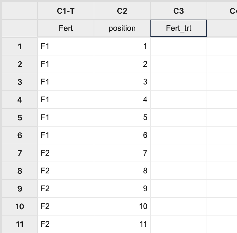
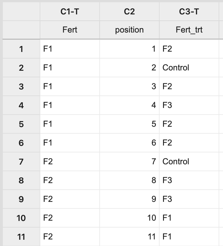
For Block 1, manually create two columns: one with each treatment level and the other with a position number 1 to n, where n is the block size (i.e. n = 4 in this example). The third column will store the assignment of fertilizer levels to the experimental units.
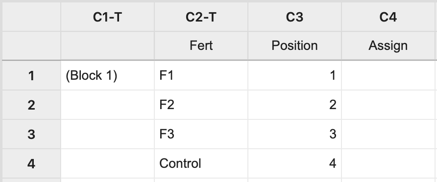
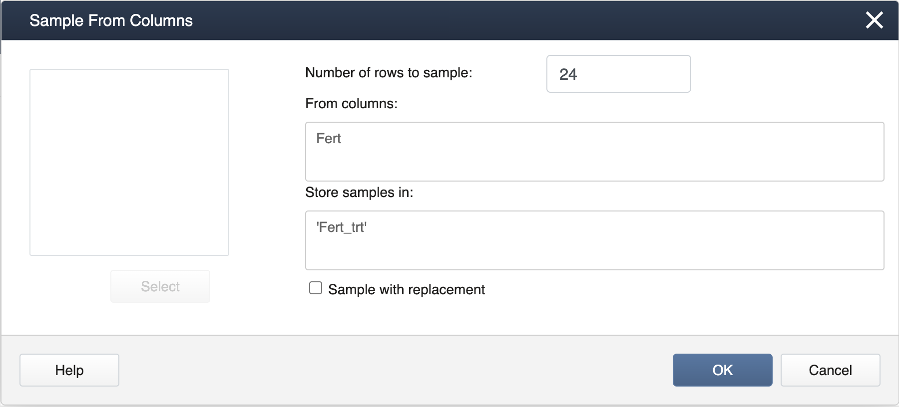
Next, select Calc > Sample from Columns > fill in the dialog box as seen below, and click OK.
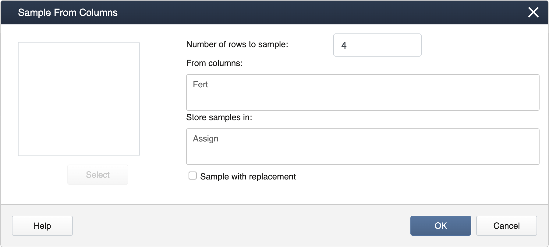
Here, the number of rows to be specified is our block size (and number of treatment levels) which yields a random assignment from Block 1.
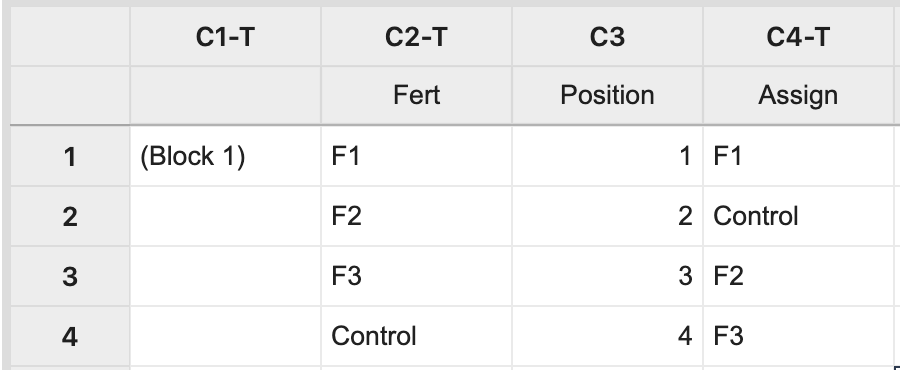
The same process should be repeated for the remaining blocks. The key element is that each treatment level or treatment combination appears in each block (forming complete blocks), and is assigned at random within each block.
To obtain the RCBD in R, we can use the blocks function from the blocksdesign package.
library(blocksdesign)
set.seed(1)
block_design = blocks(treatments = 4, replicates = 6, blocks = 6)$Design
We can then construct a data frame to view the design.
block = block_design[,1]
treatment = block_design[,3]
plant = rep(c(1:4),6)
data.frame(cbind(block,plant,treatment))
   block plant treatment
1      1     1         1
2      1     2         3
3      1     3         2
4      1     4         4
5      2     1         3
6      2     2         2
7      2     3         4
8      2     4         1
9      3     1         4
10     3     2         1
11     3     3         2
12     3     4         3
13     4     1         2
14     4     2         4
15     4     3         3
16     4     4         1
17     5     1         4
18     5     2         1
19     5     3         3
20     5     4         2
21     6     1         2
22     6     2         1
23     6     3         4
24     6     4         3
7.4 - Latin Square Design (LSD)
7.4 - Latin Square Design (LSD)The fundamental idea of blocking can be extended to more dimensions. However, the full use of multiple blocking variables in a complete block design usually requires many experimental units. Latin Square design (LSD) can be useful when we want to achieve blocking simultaneously in two directions with a limited number of experimental units.
The limitation of the Latin Square experimental layout is that the design is only possible when
number of Row blocks = number of Column blocks = number of treatments.
The experimental design process begins with a Standard Latin Square. These have the treatment levels ordered across the first row and first column. For example, consider a single factor with three levels (A, B, C), blocked in two directions resulting in this standard \(3 \times 3\) square:
| A | B | C |
| B | C | A |
| C | A | B |
To randomize, first randomly permute the order of the rows and produce a new square.
| B | C | A |
| C | A | B |
| A | B | C |
Then randomly permute the order of the columns to yield the final square for the experimental layout.
| C | A | B |
| A | B | C |
| B | C | A |
Notice that each treatment occurs only once in each row and once in each column; the fundamental requirement of a LSD. This process assures that any row or column will have all treatment levels only once.
Using Technology
To obtain the design in SAS we can use:
proc plan;
factors Row=4 ordered Col=4 ordered / noprint;
treatments Treatment=4 cyclic;
output out=LatinSquare
Row cvals=('RowBlock 1' 'RowBlock 2' 'RowBlock 3' 'RowBlock 4') random
Col cvals=('ColBlock 1' 'ColBlock 2' 'ColBlock 3' 'ColBlock 4') random
Treatment nvals=(1 2 3 4) random;
run;
The ANOVA for the Latin Square is a direct extension of the RCBD with random blocking effects. The SAS random statement has to be modified accordingly to incorporate both blocking factors and with the assumption of no interaction between them (because of only one observation for each cell). For example, we could use the following SAS code to estimate the model:
proc mixed data=LatinSquare method=type3;
class Row Col Treatment;
model Response = Treatment;
random Row Col;
run;
To obtain a Latin Square Design for four treatments we can use the function rlatin from the magic package.
library(magic)
set.seed(1)
LSD4 = rlatin(4)
LSD4
     [,1] [,2] [,3] [,4]
[1,]    4    2    3    1
[2,]    2    1    4    3
[3,]    1    3    2    4
[4,]    3    4    1    2
7.5 - Try it!
7.5 - Try it!Exercises
- A poultry experiment was run to investigate the effect of diet and antibiotics on egg production. They evaluated 2 diets of interest and 2 specific antibiotics that are on the market. The feed and antibiotic were combined and used to fill the feeding trays in barns. They chose 3 poultry farms at random and randomly assigned the combinations of diet and antibiotic to 4 barns within each farm. Total egg production by the chickens was recorded after 4 weeks.
- What is the experimental design (hint: think about the randomization process)?
- Identify which factors are fixed and which are random.
- RCBD.
- Fixed: Diet and Antibiotic; Random: Farms.
- A commercial farmer is studying the corn yield of two fertilizer types at 2 different temperature levels. He strips his cornfield into 20 strips. Each fertilizer type and temperature level combination is then assigned to 5 of the randomly chosen strips.
- What is the treatment design?
- What is the randomization design?
- 2x2 factorial with fertilizer types and temperature levels, each having 2 levels.
- CRD with 5 replicates.
- An investigator wants to run an experiment in a Latin square design evaluating 5 levels of a treatment (labeled A, B, C, D, and E) and included the layout in a research proposal that you are reviewing. Identify any problems you see and suggest how to revise the design.
A B C D E B C D B A C D E A B D E A B C E A B C D Column 4, row 2, B should be E to satisfy the property: each treatment occurs only once in each row and once in each column. In addition, the rows and columns need to be independently randomized to produce the actual layout of the Latin square for the experimental plan.
7.6 - Lesson 7 Summary
7.6 - Lesson 7 SummaryThis lesson introduced us to randomization design, which provides the scheme of how treatment levels can be assigned to experimental units. The specific designs discussed were CRD, RCBD, and Latin Square Design. An RCBD can be employed to account for a blocking factor, or nuisance variable, which is not of interest but may have an impact on the response. Likewise, a Latin square design is helpful in the presence of two such blocking variables. In an RCBD, with no replicates, the interaction between the treatment and the blocking variable is assumed to be negligible and the MS value of this interaction serves as the estimate of the error variance, which turns out to be the denominator of the F-statistic for testing treatment significance. In next lesson we will continue to learn about randomization with another widely used design; the split-plot.