9: ANCOVA Part I

Overview

An analysis of covariance (ANCOVA) procedure is used when the statistical model has both quantitative and qualitative predictors, and is based on the concepts of the General Linear Model (GLM). In ANCOVA, we combine the concepts we have learned so far in this course (applicable to categorical factors) with the principles of regression (applicable to continuous predictors, learned in STAT 501).

In this lesson, we will address the classic case of ANCOVA where the ANOVA model is extended to include the linear effect of a continuous variable, known as the covariate. In the next lesson, we will generalize the ANCOVA model to include the quadratic and cubic effects of the covariate as well.

Fun Facts: When SAS first came out they had only PROC ANOVA and PROC REGRESSION. Then people asked, "What about the case when want to do an ANOVA but have another continuous variable that you suspect will account for extraneous variability in the response?" In response, SAS came out with PROC GLM which is the general linear model. With PROC GLM you could place the continuous regression variable in the ANOVA model and it would run. Or, if you were running a regression, you could include a categorical variable in the regression model and it would also run. The GLM can handle both the regression and the categorical variables in the same model. Note, there is no PROC ANCOVA in SAS, but there is PROC MIXED. PROC GLM had problems when it came to random effects and was effectively replaced by PROC MIXED. The same sort of process was seen in Minitab and accounts for the multiple tabs under Stat > ANOVA and Stat > Regression, and eventually, Stat > General Linear Model (which works for random effects as well). So, we now have the capacity to include covariates and correctly work with random effects via SAS PROC MIXED or Minitab Stat > General Linear Model. But, enough history, let us get to this lesson.

Introduction to Analysis of Covariance (ANCOVA)

A ‘classic’ ANOVA tests for differences in mean responses to categorical factor (treatment) levels. When there is heterogeneity in experimental units, sometimes restrictions on the randomization (blocking) can improve the accuracy of significance testing results. In some situations, however, the opportunity to construct blocks may not exist, but there may exist a continuous variable causing the heterogeneity. Such sources of extraneous variability are referred to as ‘covariates’, and historically have also been termed ‘nuisance’ or ‘concomitant’ variables.

Note that an ANCOVA model is formed by including a continuous covariate in an ANOVA model. As the continuous covariate enters the model as a regression variable, an ANCOVA requires a few additional steps that should be combined with the ANOVA procedure.

Objectives

Upon completion of this lesson, you should be able to:

Be familiar with the basics of the General Linear Model (GLM) necessary for ANCOVA implementation.
Develop the ANCOVA procedure by extending the ANOVA methodology to include a continuous predictor.
Carry out the testing sequences for ANCOVA with equal and unequal slopes.

9.1 - ANCOVA in the GLM Setting: The Covariate as a Regression Variable

The statistical ANCOVA by definition is a general linear model that includes both ANOVA (categorical) predictors and regression (continuous) predictors. The simple linear regression model is:

\(Y_i=\beta_0+\beta_1 X_i+ \epsilon_i\)

Here, \(\beta_0\) and \(\beta_1\) are the intercept and the slope of the line, respectively. The significance of a regression is equivalent to testing \(H_0 \colon \beta_1=0 \text{ vs. } H_1\colon \beta_1 \neq 0\) using the \(\text{F-statistic} = \frac{MS(Regr)}{MSE}\) where \(MS(Regr)\) is the mean sum of squares for regression and MSE is the mean squared error. In this case of a simple linear regression, the F-test is equivalent to a t-test.

Now, in adding the regression variable to our one-way ANOVA model, we can envision a notational problem. In the balanced one-way ANOVA, we have the grand mean (\(\mu\)), but now we also have the intercept \(\beta_0\). To get around this, we can use

\(X^*=X_{ij}-\bar{X}_{..}\)

and get the following as an expression of our covariance model:

\(Y_{ij}=\mu+\tau_i+\gamma X^* +\epsilon_{ij}\)

Note, in a GLM, the Type III (model fit) sums of squares for the treatment levels are being corrected (or adjusted) for the regression relationship. This has the effect of evaluating the treatment levels ‘on the same playing field’. That is, comparing the means of the treatment levels at the mean value of the covariate. This process effectively removes the variation due to the covariate that may otherwise be attributed to treatment level differences.

9.2 - Steps in ANCOVA

First, we need to confirm that for at least one of the treatment groups there is a significant regression relationship with the covariate. Otherwise, including the covariate in the model won’t improve the estimation of treatment means.

Once this is confirmed, we need to examine whether the regression relationship between the response and the covariate has the same slope for each treatment group. Graphically, this means that the regression line at each factor level has the same slope and therefore the lines are all parallel.

Depending on the outcome of the test for equal slopes, we have two alternative ways to finish up the ANCOVA:

Fit a common slope model and adjust the treatment SS for the presence of the covariate.
Evaluate the differences in means for at least three levels of the covariate.

These steps are illustrated in the following two sections and are diagrammed below:

Note! The figure above is presented as a guideline and does require some subjective judgment. Small sample sizes, for example, may result in none of the individual regressions in Step 1 being statistically significant. Yet, the inclusion of the covariate in the model may still be advantageous as pooling the data will increase the number of observations when fitting the joint model. Exploratory data analysis and regression diagnostics also will be useful.

9.3 - Comparison to ANOVA: Salary Example

To illustrate the role the covariate has in the ANCOVA, let’s look at a hypothetical situation wherein investigators are comparing the salaries of male vs. female college graduates. A random sample of 5 individuals for each gender is compiled, and a simple one-way ANOVA is performed:

Males	Females
78	80
43	50
103	30
48	20
80	60

\(H_0 \colon \mu_{\text{ Males}}=\mu_{\text{ Females}}\)

SAS coding for the one-way ANOVA:

data ancova_example;
input gender $ salary;
datalines;
m 78
m 43
m 103
m 48
m 80
f 80
f 50
f 30
f 20
f 60
;
proc mixed data=ancova_example method=type3;
class gender;
model salary=gender;
run;

Here is the output we get:

Type 3 Tests of Fixed Effects
Effect	Num DF	Den DF	F Value	Pr > F
gender	1	8	2.11	0.1840

To perform a one-way ANOVA test in Minitab, you can first open the data (ANCOVA Example Minitab Data) and then select Stat > ANOVA > One Way…

In the pop-up window that appears, select salary as the Response and gender as the Factor.

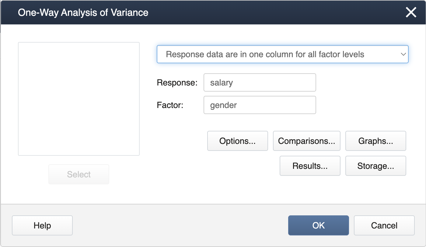
Click OK, and the output is as follows.

Analysis of Variance

Source	DF	SS	SS	F-Value	P-Value
gender	1	1254	1254	2.11	0.184
Error	8	4745	593
Total	9	6000

Model Summary

S	R-sq	R-sq(adj)	R-sq(pred)
24.3547	20.91%	11.02%	0.00%

First, we can input the data manually for such a small dataset.

gender = c(rep("m",5),rep("f",5))
salary = c(78,43,103,48,80,80,50,30,20,60)

We then apply a simple one-way ANOVA and display the ANOVA table.

Anova Table (Type III tests)

Response: salary
             Sum Sq Df  F value     Pr(>F)    
(Intercept) 35046.4  1 59.08522 5.8151e-05 ***
gender       1254.4  1  2.11481    0.18396    
Residuals    4745.2  8                        
---
Signif. codes:  0 ‘***’ 0.001 ‘**’ 0.01 ‘*’ 0.05 ‘.’ 0.1 ‘ ’ 1

9.4 - Equal Slopes Model: Salary Example

Using Technology

Using our Salary example and the data in the table below, we can run through the steps for the ANCOVA.

Females		Males
Salary	Years	Salary	Years
80	5	78	3
50	3	43	1
30	2	103	5
20	1	48	2
60	4	80	4

Step 1: Are all regression slopes = 0?

A simple linear regression can be run for each treatment group, Males and Females. Running these procedures using statistical software we get the following:

Males

Use the following SAS code:

data equal_slopes;
input gender $ salary years;
datalines;
m 78 3
m 43 1
m 103 5
m 48 2
m 80 4
f 80 5
f 50 3
f 30 2
f 20 1
f 60 4
;
proc reg data=equal_slopes;
where gender='m';
model salary=years;
title 'Males';
run; quit;

And here is the output that you get:

The REG Procedure Mode1:: MODEL1 Dependent Variable: salary
Number of Observations Read	5
Number of Observations Used	5

Analysis of Variance
Source	DF	Sum of Squares	Mean Square	F Value	Pr > F
Model	1	2310.40000	2310.40000	44.78	0.0068
Error	3	154.80000	51.60000
Corrected Total	4	2465.20000

Females

Use the following SAS code:

data equal_slopes;
input gender $ salary years;
datalines;
m 78 3
m 43 1
m 103 5
m 48 2
m 80 4
f 80 5
f 50 3
f 30 2
f 20 1
f 60 4
;
proc reg data=equal_slopes;
where gender='f';
model salary=years;
title 'Females';
run; quit;

And here is the output for this run:

The REG Procedure Mode1:: MODEL1 Dependent Variable: salary
Number of Observations Read	5
Number of Observations Used	5

Analysis of Variance
Source	DF	Sum of Squares	Mean Square	F Value	Pr > F
Model	1	2250.00000	2250.00000	225.00	0.0006
Error	3	30.00000	10.00000
Corrected Total	4	2280.00000

In both cases, the simple linear regressions are significant so the slopes are not = 0.

Step 2: Are the slopes equal?

We can test for this using our statistical software.

In SAS we now use proc mixed and include the covariate in the model.

We will also include a ‘treatment × covariate’ interaction term and the significance of this term answers our question. If the slopes differ significantly among treatment levels, the interaction p-value will be < 0.05.

data equal_slopes;
input gender $ salary years;
datalines;
m 78 3
m 43 1
m 103 5
m 48 2
m 80 4
f 80 5
f 50 3
f 30 2
f 20 1
f 60 4
;
proc mixed data=equal_slopes method=type3;
class gender;
model salary = gender years gender*years;
run;

Note! In SAS, we specify the treatment in the class statement, indicating that these are categorical levels. By NOT including the covariate in the class statement, it will be treated as a continuous variable for regression in the model statement.

The Mixed Procedure Type 3 Tests of Fixed Effects
Effect	Num DF	Den DF	F Value	Pr > F
years	1	6	148.06	<.0001
gender	1	6	7.01	0.0381
years*gender	1	6	0.01	0.9384

Here we see that the slopes are equal and in a plot of the regressions, we see that the lines are parallel.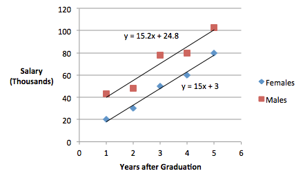

To obtain the plot in SAS, we can use the following SAS code:

ods graphics on;
proc sgplot data=equal_slopes;
styleattrs datalinepatterns=(solid);
reg y=salary x=years / group=gender;
run;

Step 3: Fit an Equal Slopes Model

We can now proceed to fit an Equal Slopes model by removing the interaction term. Again, we will use our statistical software SAS.

data equal_slopes;
input gender $ salary years;
datalines;
m 78 3
m 43 1
m 103 5
m 48 2
m 80 4
f 80 5
f 50 3
f 30 2
f 20 1
f 60 4
;
proc mixed data=equal_slopes method=type3;
class gender;
model salary = gender years;
lsmeans gender / pdiff adjust=tukey;
/* Tukey unnecessary with only two treatment levels */
title 'Equal Slopes Model';
run;

We obtain the following results:

The Mixed Procedure Type 3 Tests of Fixed Effects
Effect	Num DF	Den DF	F Value	Pr > F
years	1	7	172.55	<.0001
gender	1	7	47.46	0.0002

Least Squares Means
Effect	gender	Estimate	Standard Error	DF	t Value	Pr > \|t\|
gender	f	48.0000	2.2991	7	20.88	<.0001
gender	m	70.4000	2.2991	7	30.62	<.0001

Note! In SAS, the model statement automatically creates an intercept. This produces the correct table for testing the effects (using the adjusted sum of squares). However, including the intercept technically over-parameterizes the ANCOVA model resulting in an additional calculation step to obtain the regression equations. To get the intercepts for the covariate directly, we can re-parameterize the model by suppressing the intercept (noint) and then specifying that we want the solutions (solution) to the model. However, this should only be done to find the equation estimates, not to test effects.

Here is what the SAS code looks like for this:

data equal_slopes;
input gender $ salary years;
datalines;
m 78 3
m 43 1
m 103 5
m 48 2
m 80 4
f 80 5
f 50 3
f 30 2
f 20 1
f 60 4
;
proc mixed data=equal_slopes method=type3;
class gender;
model salary = gender years / noint solution;
ods select SolutionF;
title 'Equal Slopes Model';
run;

Here is the output:

Solution for Fixed Effects
Effect	gender	Estimate	Standard Error	DF	t Value	Pr > \|t\|
gender	f	2.7000	4.1447	7	0.65	0.5356
gender	m	25.1000	4.1447	7	6.06	0.0005
years		15.1000	1.1495	7	13.14	<.0001

In the first section of the output above a separate intercept is reported for each gender, the ‘Estimate’ value for each gender, and a common slope for both genders, labeled ‘Years’.

Thus, the estimated regression equation for Females is \(\hat{y} = 2.7 + 15.1 \text{(Years)}\), and for males it is \(\hat{y} = 25.1 + 15.1 \text{(Years)}\)

To this point in this analysis, we can see that 'gender' is now significant. By removing the impact of the covariate, we went from

Type 3 Tests of Fixed Effects
Effect	Num DF	Den DF	F Value	Pr > F
gender	1	8	2.11	0.1840

(without covariate consideration)

gender	1	7	47.46	0.0002

(adjusting for the covariate)

Using our Salary example and the data in the table below, we can run through the steps for the ANCOVA. On this page, we will go through the steps using Minitab.

Females		Males
Salary	Years	Salary	Years
80	5	78	3
50	3	43	1
30	2	103	5
20	1	48	2
60	4	80	4

Step 1: Are all regression slopes = 0?

A simple linear regression can be run for each treatment group, Males and Females. To perform regression analysis on each gender group in Minitab, we will have to subdivide the salary data manually and separately, saving the male data into the Male Salary Dataset and the female data into the Female Salary dataset.

Running these procedures using statistical software we get the following:

Males

Open the Male dataset in the Minitab project file (Male Salary Dataset).

Then, from the menu bar, select Stat > Regression > Regression > Fit Regression Model

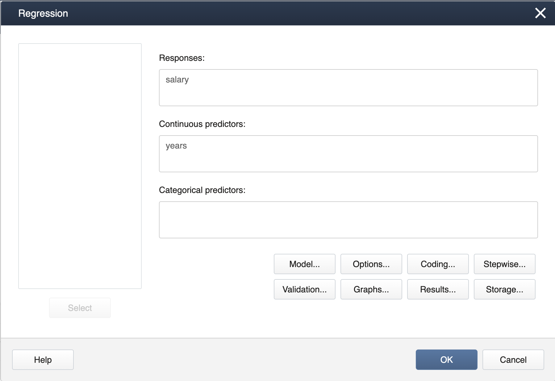
In the pop-up window, select salary into Response and years into Predictors as shown below.

Minitab Regression window with Responses=salary, Continuous predictors=years

Click OK, and Minitab will output the following.

Regression Analysis: Salary versus years

Regression Equation

salary = 24.8 + 15.2 years

Coefficients

Term	Coef	SE Coef	T-Value	P-Value	VIF
Constant	24.80	7.53	3.29	0.046
years	15.20	2.27	6.69	0.007	1.00

Model Summary

S	R-sq	R-sq(adj)	R-sq(pred)
7.18331	R-Sq = 93.7%	91.6%	85.94%

Analysis of Variance

Source	DF	SS	MS	F-Value	P-Value
Regression	1	2310.4	2310.40	44.78	0.007
years	1	2310.4	2310.40	44.78	0.007
Residual Error	3	154.8	51.6
Total	4	2465.2

Females

Open Minitab dataset Female Salary Dataset. Follow the same procedure as was done for the Male dataset and Minitab will output the following:

Regression Analysis: Salary versus years

Regression Equation

salary = 3.00 + 15.00 years

Coefficients

Term	Coef	SE Coef	T-Value	P-Value	VIF
Constant	3.00	3.32	0.90	0.432
years	15.00	1.00	15.00	0.001	1.00

Model Summary

S	R-sq	R-sq(adj)	R-sq(pred)
3.16228	98.68%	98.25%	95.92%

Analysis of Variance

Source	DF	SS	MS	F-Value	P-Value
Regression	1	2250.0	2250.0	225.00	0.001
years	1	2250.0	2250.0	225.00	0.001
Residual Error	3	30.0	10.0
Total	4	2280.0

In both cases, the simple linear regressions are significant, so the slopes are not = 0.

Step 2: Are the slopes equal?

We can test for this using our statistical software. In Minitab, we must now use GLM (general linear model) and be sure to include the covariate in the model. We will also include a ‘treatment x covariate’ interaction term and the significance of this term is what answers our question. If the slopes differ significantly among treatment levels, the interaction p-value will be < 0.05.

First, open the dataset in the Minitab project file Salary Dataset. Then, from the menu select Stat > ANOVA > General Linear Model > Fit General Linear Model

In the dialog box, select salary into Responses, gender into Factors, and years into Covariates.

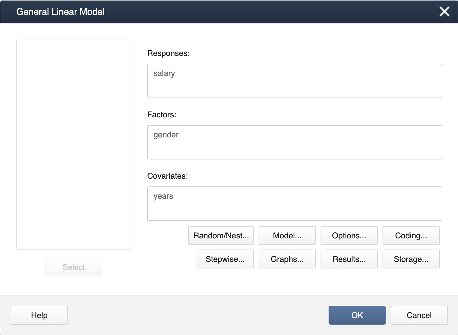
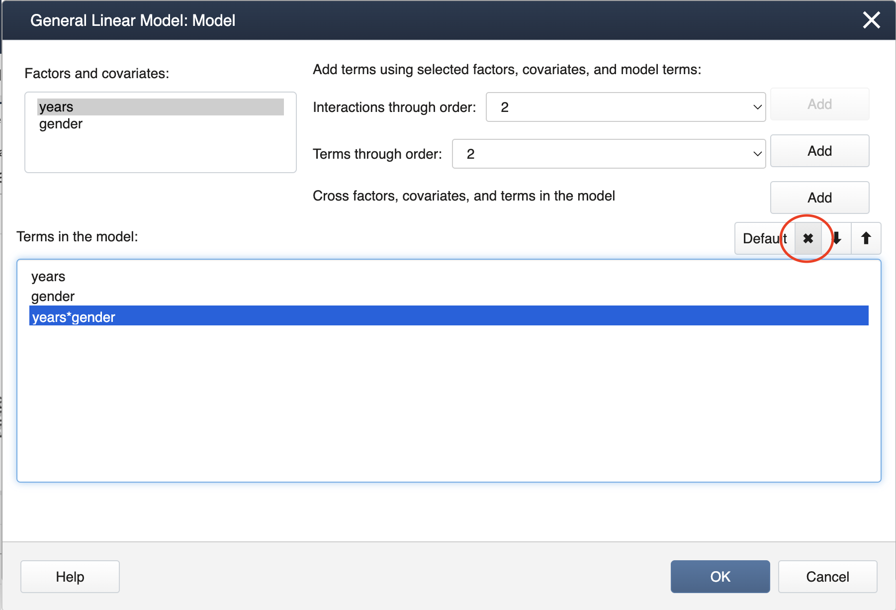
Minitab General Linear Model window with Responses= salary, Factors=gender and Covariates=years

To add the interaction term, first click Model…. Then, use the shift key to highlight gender and years, and click Add. Click OK, then OK again, and Minitab will display the following output.

Analysis of Variance

Source	DF	Adj SS	Adj MS	F-Value	P-Value
year	1	4560.20	4560.20	148.06	0.000
gender	1	216.02	216.02	7.01	0.038
years*gender	1	0.20	0.20	0.01	0.938
Error	6	184.80	30.80
Total	9	5999.60

It is clear the interaction term is not significant. This suggests the slopes are equal. In a plot of the regressions, we can also see that the lines are parallel.

Step 3: Fit an Equal Slopes Model

We can now proceed to fit an Equal Slopes model by removing the interaction term. This can be easily accomplished by starting again with STAT > ANOVA > General Linear Model > Fit General Linear Model

Click OK, then OK again, and Minitab will display the following output.

Analysis of Variance

Source	DF	Adj SS	Adj MS	F-Value	P-Value
year	1	4560.20	4560.20	172.55	0.000
gender	1	1254.4	1254.40	47.46	0.000
Error	7	185.0	26.43
Total	9	5999.6

To generate the mean comparisons select STAT > ANOVA > General Linear Model > Comparisons... and fill in the dialog box as seen below.

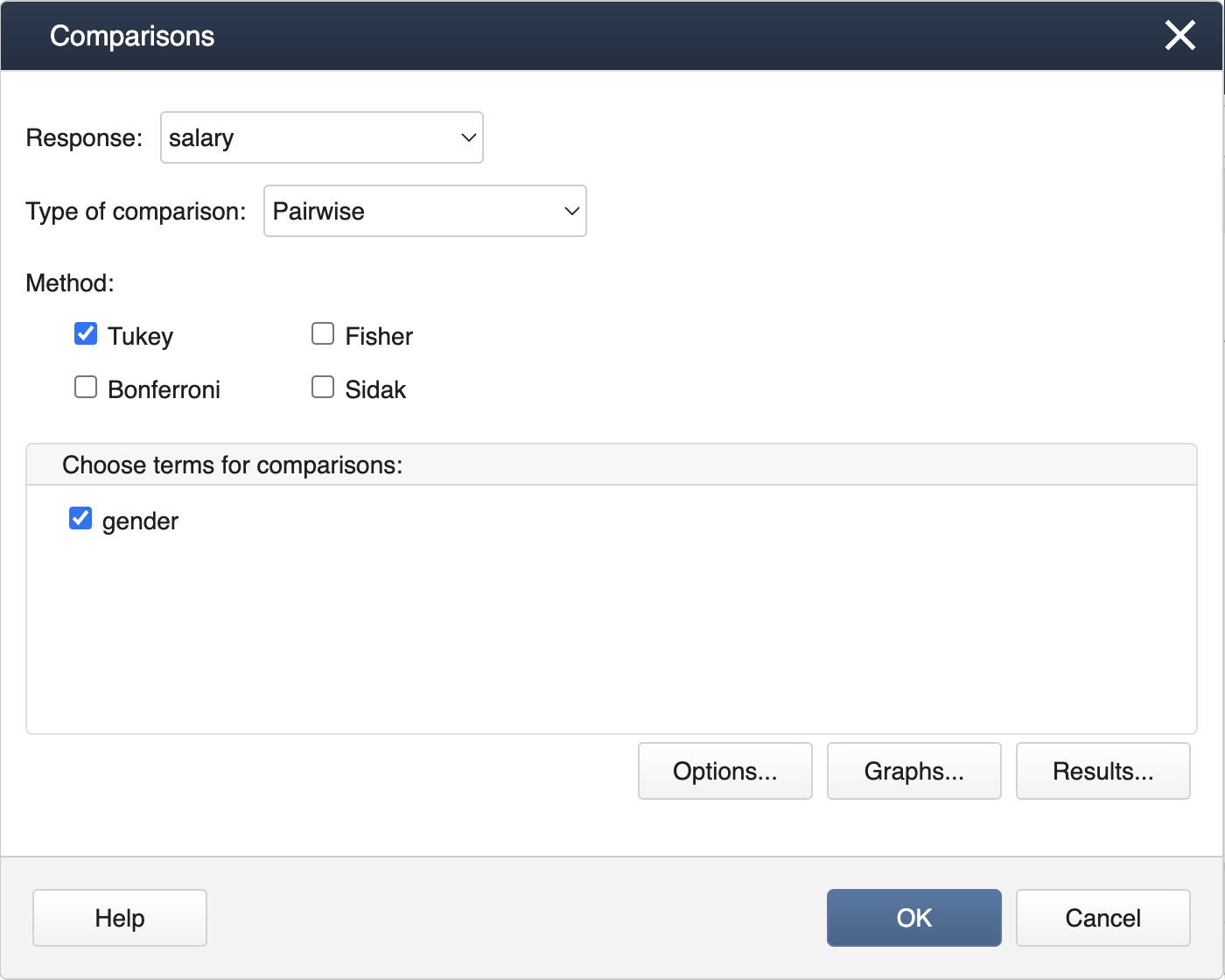
Minitab Comparisions windo with Response=salary, Type of Comparison=Pairwise and Method= Tukey

Click OK and Minitab will produce the following output.

Comparison of salary

Tukey Pairwise Comparisons: gender

Grouping information Using the Tukey Method and 95% Confidence

gender N Mean Grouping
Male 5 70.4 A
gender 5 48.0 B
Means that do not share a letter are significantly different.

gender	N	Mean	Grouping
Male	5	70.4	A
gender	5	48.0	B

First, we can input the data manually.

gender = c(rep("m",5),rep("f",5))
salary = c(78,43,103,48,80,80,50,30,20,60)
years = c(3,1,5,2,4,5,3,2,1,4)
salary_data = data.frame(salary,gender,years)

We can apply a simple linear regression for the male subset of the data and display the results using summary.

male_data = subset(salary_data,gender=="m")
lm_male = lm(salary~years,male_data)
summary(lm_male)

Call:
lm(formula = salary ~ years, data = male_data)

Residuals:
   1    2    3    4    5 
 7.6  3.0  2.2 -7.2 -5.6 

Coefficients:
            Estimate Std. Error t value Pr(>|t|)   
(Intercept)   24.800      7.534   3.292  0.04602 * 
years         15.200      2.272   6.691  0.00681 **
---
Signif. codes:  0 ‘***’ 0.001 ‘**’ 0.01 ‘*’ 0.05 ‘.’ 0.1 ‘ ’ 1

Residual standard error: 7.183 on 3 degrees of freedom
Multiple R-squared:  0.9372,	Adjusted R-squared:  0.9163 
F-statistic: 44.78 on 1 and 3 DF,  p-value: 0.006809

Next, we apply a simple linear regression for the female subset.

female_data = subset(salary_data,gender=="f")
lm_female = lm(salary~years,female_data)
summary(lm_female)

Call:
lm(formula = salary ~ years, data = female_data)

Residuals:
 6  7  8  9 10 
 2  2 -3  2 -3 

Coefficients:
            Estimate Std. Error t value Pr(>|t|)    
(Intercept)    3.000      3.317   0.905 0.432389    
years         15.000      1.000  15.000 0.000643 ***
---
Signif. codes:  0 ‘***’ 0.001 ‘**’ 0.01 ‘*’ 0.05 ‘.’ 0.1 ‘ ’ 1

Residual standard error: 3.162 on 3 degrees of freedom
Multiple R-squared:  0.9868,	Adjusted R-squared:  0.9825 
F-statistic:   225 on 1 and 3 DF,  p-value: 0.0006431

It is clear the regression for both treatments is significant. We continue to test for unequal slopes in the full dataset using an interaction term.

options(contrasts=c("contr.sum","contr.poly"))
lm_unequal = lm(salary~gender+years+gender:years,salary_data)
aov3_unequal = car::Anova(lm_unequal,type=3)
aov3_unequal

Anova Table (Type III tests)

Response: salary
             Sum Sq Df  F value    Pr(>F)    
(Intercept)   351.3  1  11.4055   0.01491 *  
gender        216.0  1   7.0136   0.03811 *  
years        4560.2  1 148.0584 1.874e-05 ***
gender:years    0.2  1   0.0065   0.93839    
Residuals     184.8  6                       
---
Signif. codes:  0 ‘***’ 0.001 ‘**’ 0.01 ‘*’ 0.05 ‘.’ 0.1 ‘ ’ 1

The interaction term is not significant, suggesting the slopes do not differ significantly. We simplify the model to the equal-slope model without an interaction term.

lm_equal = lm(salary~gender+years,salary_data)
aov3_equal = car::Anova(lm_equal,type=3)
aov3_equal

Anova Table (Type III tests)

Response: salary
            Sum Sq Df F value    Pr(>F)    
(Intercept)  351.3  1  13.292 0.0082232 ** 
gender      1254.4  1  47.464 0.0002335 ***
years       4560.2  1 172.548 3.458e-06 ***
Residuals    185.0  7                      
---
Signif. codes:  0 ‘***’ 0.001 ‘**’ 0.01 ‘*’ 0.05 ‘.’ 0.1 ‘ ’ 1

This is the final model since all terms are significant. We can then produce the LS means for the gender levels.

aov1_equal = aov(lm_equal)
lsmeans_gender = emmeans::emmeans(aov1_equal,~gender) 
lsmeans_gender

 gender emmean  SE df lower.CL upper.CL
 f        48.0 2.3  7     42.6     53.4
 m        70.4 2.3  7     65.0     75.8

Confidence level used: 0.95

We can also find the regression equation coefficients. Note the female level was used as the reference level by default.

  aov1_equal$coefficients

(Intercept)     genderm       years 
        2.7        22.4        15.1

9.5 - Unequal Slopes Model: Salary Example

Using Technology

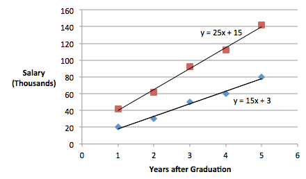
If the data collected in the example study were instead as follows:

Females		Males
Salary	Years	Salary	Years
80	5	42	1
50	3	112	4
30	2	92	3
20	1	62	2
60	4	142	5

We would see in Step 2 that we do have a significant 'treatment × covariate' interaction. Using SAS we can run the unequal slope model.

data unequal_slopes;
input gender $ salary years;
datalines;
m  42  1
m  112  4
m  92  3
m  62  2
m  142  5
f  80  5
f  50  3
f  30  2
f  20  1
f  60  4
;
proc mixed data=unequal_slopes method=type3;
class gender;
model salary=gender years gender*years;
title 'Covariance Test for Equal Slopes';
/*Note that we found a significant years*gender interaction*/
/*so we add the lsmeans for comparisons*/
/*With 2 treatments levels we omitted the Tukey adjustment*/
lsmeans gender/pdiff at years=1;
lsmeans gender/pdiff at years=3;
lsmeans gender/pdiff at years=5;
run;

We get the following output:

Type 3 Test of Fixed Effects
Effect	Num DF	De DF	F Value	Pr > F
years	1	6	800.00	< .0001
gender	1	6	6.55	0.0430
years*gender	1	6	50.00	0.0004

To generate the covariate regression slopes and intercepts, we can do the following.

data unequal_slopes;
input gender $ salary years;
datalines;
m  42  1
m  112  4
m  92  3
m  62  2
m  142  5
f  80  5
f  50  3
f  30  2
f  20  1
f  60  4
;
proc mixed data=unequal_slopes method=type3;
class gender;
model salary=gender years gender*years / noint solution;
ods select SolutionF;
title 'Reparmeterized Model';
run;

This produces the following output:

Solution for Fixed Effects
Effect	gender	Estimate	Standard Error	DF	t Value	Pr > \|t\|
gender	f	3.0000	3.3166	6	0.90	0.4006
gender	m	15.0000	3.3166	6	4.52	0.0040
years		25.0000	1.0000	6	25.00	<.0001
years*gender	f	-10.0000	1.4142	6	-7.07	0.0004
years*gender	m	0	.	.	.	.

Here the intercepts are the estimates for effects labeled 'gender' and the slopes can be derived from the estimates of the effects labeled 'years' and 'years*gender'. Thus, the regression equations for this unequal slopes model are:

\(\text{Females}\;\;\; \hat{y} = 3.0 + 15(Years)\)

\(\text{Males}\;\;\; \hat{y} = 15 + 25(Years)\)

The slopes of the regression lines differ significantly and are not parallel.

The code above also outputs the following:

Differences of Least Squares Means
Effect	gender	_gender	years	Estimate	Standard Error	DF	t Value	Pr > \|t\|
gender	f	m	1.00	-22.000	3.4641	6	-6.35	0.0007
gender	f	m	3.00	-42.000	2.0000	6	-21.00	< .0001
gender	f	m	5.00	-62.000	3.4641	6	-17.90	< .0001

In this case, we see a significant difference at each level of the covariate specified in the lsmeans statement. The magnitude of the difference between males and females differs, giving rise to the significant interaction. In more realistic situations, a significant 'treatment × covariate' interaction often results in significant treatment level differences at certain points along the covariate axis.

When we re-run the program with the new dataset Salary-new Data, we find a significant interaction between gender and years.

To do this, open the Minitab dataset Salary-new Data.

Go to Stat > ANOVA > General Linear model > Fit General Linear Model and follow the same sequence of steps as in the previous section. In Step 2, Minitab will display the following output.

Analysis of Variance

Source	DF	Adj SS	Adj MS	F-Value	P-Value
years	1	8000.0	8000.0	800.00	0.000
gender	1	65.5	65.45	6.55	0.043
years*gender	1	500.0	500.0	50.00	0.000
Error	6	60.0	10.00
Total	9	12970.0

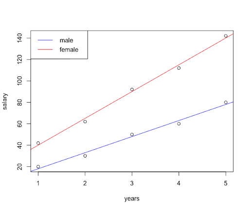
It is clear the interaction term is significant and should not be removed. This suggests the slopes are not equal. Thus, the magnitude of the difference between males and females differs (giving rise to the interaction significance).

First, we can input the data manually.

gender = c(rep("m",5),rep("f",5))
salary = c(42,112,92,62,142,80,50,30,20,60)
years = c(1,4,3,2,5,5,3,2,1,4)
salary_data = data.frame(salary,gender,years)

If we were to fit regression models for both gender treatments we would see both regressions are significant. We then test for unequal slopes in the full dataset using an interaction term.

options(contrasts=c("contr.sum","contr.poly"))
lm_unequal3 = lm(salary~gender+years+gender:years,salary_data)
aov3_unequal = car::Anova(lm_unequal3,type=3)
aov3_unequal

Anova Table (Type III tests)

Response: salary
             Sum Sq Df  F value    Pr(>F)    
(Intercept)   147.3  1  14.7273 0.0085827 ** 
gender         65.5  1   6.5455 0.0430007 *  
years        8000.0  1 800.0000 1.293e-07 ***
gender:years  500.0  1  50.0000 0.0004009 ***
Residuals      60.0  6                       
---
Signif. codes:  0 ‘***’ 0.001 ‘**’ 0.01 ‘*’ 0.05 ‘.’ 0.1 ‘ ’ 1

The interaction term is significant, suggesting the slopes differ significantly. This is the final model since all terms are significant. We can then produce regression equation coefficients. To match SAS, we utilize dummy coding. Note the female level was used as the reference level by default.

options(contrasts=c("contr.treatment","contr.poly"))
lm_unequal1 = lm(salary~gender+years+gender:years,salary_data)
aov1_unequal = aov(lm_unequal1)
aov1_unequal$coefficients

  (Intercept)       genderm         years genderm:years 
            3            12            15            10

We can also plot the regression lines for both treatments.

plot(years,salary)
abline(lm(salary~years,data=subset(salary_data,gender=="m")),col="red")
abline(lm(salary~years,data=subset(salary_data,gender=="f")),col="blue")
legend("topleft",legend = c("male","female"),col=c("blue","red"),lty=1)

Finally, we can find the differences in the treatment LS means for various years (1, 3, and 5).

lsmeans_gender1 = emmeans::emmeans(aov1_unequal,pairwise~gender|years,at=list(years=1)) 
lsmeans_gender1$contrasts

lsmeans_gender3 = emmeans::emmeans(aov1_unequal,pairwise~gender|years,at=list(years=3)) 
lsmeans_gender3$contrasts

lsmeans_gender5 = emmeans::emmeans(aov1_unequal,pairwise~gender|years,at=list(years=5)) 
lsmeans_gender5$contrasts

years = 1:
 contrast estimate   SE df t.ratio p.value
 f - m         -22 3.46  6  -6.351  0.0007

years = 3:
 contrast estimate SE df t.ratio p.value
 f - m         -42  2  6 -21.000  <.0001

years = 5:
 contrast estimate   SE df t.ratio p.value
 f - m         -62 3.46  6 -17.898  <.0001

9.6 - Lesson 9 Summary

This lesson introduced us to ANCOVA methodology, which accommodates both continuous and categorical predictors. The model discussed in this lesson had one categorical factor and a linear effect of one covariate, the continuous predictor. We noted that the fitted linear relationship between the response and the covariate resulted in a straight line for each factor level, and the ANCOVA procedure depended on the condition of equal (or unequal) slopes. We saw one advantage of ANCOVA was the ability to examine the differences among the factor levels after adjusting for the impact of the covariate on the response.

The salary example comparing males and females after accounting for their years after college illustrated how software can be utilized when using the ANCOVA procedure. In the next lesson, the ANCOVA topic will be extended to include in the model up to a cubic polynomial relationship between response vs covariate.

^[1]	Link
↥	Has Tooltip/Popover
	Toggleable Visibility

9: ANCOVA Part I

Overview

Introduction to Analysis of Covariance (ANCOVA)

Objectives

9.1 - ANCOVA in the GLM Setting: The Covariate as a Regression Variable

9.2 - Steps in ANCOVA

9.3 - Comparison to ANOVA: Salary Example

Analysis of Variance

Model Summary

9.4 - Equal Slopes Model: Salary Example

Using Technology

Step 1: Are all regression slopes = 0?

Males

Females

Step 2: Are the slopes equal?

Step 3: Fit an Equal Slopes Model

Step 1: Are all regression slopes = 0?

Males

Regression Analysis: Salary versus years

Regression Equation

Coefficients

Model Summary

Analysis of Variance

Females

Regression Analysis: Salary versus years

Regression Equation

Coefficients

Model Summary

Analysis of Variance

Step 2: Are the slopes equal?

Analysis of Variance

Step 3: Fit an Equal Slopes Model

Analysis of Variance

Comparison of salary

Tukey Pairwise Comparisons: gender

Grouping information Using the Tukey Method and 95% Confidence

9.5 - Unequal Slopes Model: Salary Example

Using Technology

Analysis of Variance

9.6 - Lesson 9 Summary