9.5 - Unequal Slopes Model: Salary Example
9.5 - Unequal Slopes Model: Salary Example
Using Technology
If the data collected in the example study were instead as follows:
| Females | Males | ||
|---|---|---|---|
| Salary | Years | Salary | Years |
| 80 | 5 | 42 | 1 |
| 50 | 3 | 112 | 4 |
| 30 | 2 | 92 | 3 |
| 20 | 1 | 62 | 2 |
| 60 | 4 | 142 | 5 |
We would see in Step 2 that we do have a significant 'treatment × covariate' interaction. Using SAS we can run the unequal slope model.
data unequal_slopes;
input gender $ salary years;
datalines;
m  42  1
m  112  4
m  92  3
m  62  2
m  142  5
f  80  5
f  50  3
f  30  2
f  20  1
f  60  4
;
proc mixed data=unequal_slopes method=type3;
class gender;
model salary=gender years gender*years;
title 'Covariance Test for Equal Slopes';
/*Note that we found a significant years*gender interaction*/
/*so we add the lsmeans for comparisons*/
/*With 2 treatments levels we omitted the Tukey adjustment*/
lsmeans gender/pdiff at years=1;
lsmeans gender/pdiff at years=3;
lsmeans gender/pdiff at years=5;
run;
We get the following output:
| Type 3 Test of Fixed Effects | ||||
|---|---|---|---|---|
| Effect | Num DF | De DF | F Value | Pr > F |
| years | 1 | 6 | 800.00 | < .0001 |
| gender | 1 | 6 | 6.55 | 0.0430 |
| years*gender | 1 | 6 | 50.00 | 0.0004 |
To generate the covariate regression slopes and intercepts, we can do the following.
data unequal_slopes;
input gender $ salary years;
datalines;
m  42  1
m  112  4
m  92  3
m  62  2
m  142  5
f  80  5
f  50  3
f  30  2
f  20  1
f  60  4
;
proc mixed data=unequal_slopes method=type3;
class gender;
model salary=gender years gender*years / noint solution;
ods select SolutionF;
title 'Reparmeterized Model';
run;
This produces the following output:
| Solution for Fixed Effects | ||||||
|---|---|---|---|---|---|---|
| Effect | gender | Estimate | Standard Error | DF | t Value | Pr > |t| |
| gender | f | 3.0000 | 3.3166 | 6 | 0.90 | 0.4006 |
| gender | m | 15.0000 | 3.3166 | 6 | 4.52 | 0.0040 |
| years | 25.0000 | 1.0000 | 6 | 25.00 | <.0001 | |
| years*gender | f | -10.0000 | 1.4142 | 6 | -7.07 | 0.0004 |
| years*gender | m | 0 | . | . | . | . |
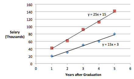
Here the intercepts are the estimates for effects labeled 'gender' and the slopes can be derived from the estimates of the effects labeled 'years' and 'years*gender'. Thus, the regression equations for this unequal slopes model are:
\(\text{Females}\;\;\; \hat{y} = 3.0 + 15(Years)\)
\(\text{Males}\;\;\; \hat{y} = 15 + 25(Years)\)
The slopes of the regression lines differ significantly and are not parallel.
The code above also outputs the following:
|
Differences of Least Squares Means |
||||||||
|---|---|---|---|---|---|---|---|---|
| Effect | gender | _gender | years | Estimate | Standard Error | DF | t Value | Pr > |t| |
| gender | f | m | 1.00 | -22.000 | 3.4641 | 6 | -6.35 | 0.0007 |
| gender | f | m | 3.00 | -42.000 | 2.0000 | 6 | -21.00 | < .0001 |
| gender | f | m | 5.00 | -62.000 | 3.4641 | 6 | -17.90 | < .0001 |
In this case, we see a significant difference at each level of the covariate specified in the lsmeans statement. The magnitude of the difference between males and females differs, giving rise to the significant interaction. In more realistic situations, a significant 'treatment × covariate' interaction often results in significant treatment level differences at certain points along the covariate axis.
When we re-run the program with the new dataset Salary-new Data, we find a significant interaction between gender and years.
To do this, open the Minitab dataset Salary-new Data.
Go to Stat > ANOVA > General Linear model > Fit General Linear Model and follow the same sequence of steps as in the previous section. In Step 2, Minitab will display the following output.
Analysis of Variance
| Source | DF | Adj SS | Adj MS | F-Value | P-Value |
|---|---|---|---|---|---|
| years | 1 | 8000.0 | 8000.0 | 800.00 | 0.000 |
| gender | 1 | 65.5 | 65.45 | 6.55 | 0.043 |
| years*gender | 1 | 500.0 | 500.0 | 50.00 | 0.000 |
| Error | 6 | 60.0 | 10.00 | ||
| Total | 9 | 12970.0 |
It is clear the interaction term is significant and should not be removed. This suggests the slopes are not equal. Thus, the magnitude of the difference between males and females differs (giving rise to the interaction significance).
First, we can input the data manually.
gender = c(rep("m",5),rep("f",5))
salary = c(42,112,92,62,142,80,50,30,20,60)
years = c(1,4,3,2,5,5,3,2,1,4)
salary_data = data.frame(salary,gender,years)
If we were to fit regression models for both gender treatments we would see both regressions are significant. We then test for unequal slopes in the full dataset using an interaction term.
options(contrasts=c("contr.sum","contr.poly"))
lm_unequal3 = lm(salary~gender+years+gender:years,salary_data)
aov3_unequal = car::Anova(lm_unequal3,type=3)
aov3_unequal
Anova Table (Type III tests)

Response: salary
             Sum Sq Df  F value    Pr(>F)
(Intercept)   147.3  1  14.7273 0.0085827 **
gender         65.5  1   6.5455 0.0430007 *
years        8000.0  1 800.0000 1.293e-07 ***
gender:years  500.0  1  50.0000 0.0004009 ***
Residuals      60.0  6
---
Signif. codes:  0 ‘***’ 0.001 ‘**’ 0.01 ‘*’ 0.05 ‘.’ 0.1 ‘ ’ 1
The interaction term is significant, suggesting the slopes differ significantly. This is the final model since all terms are significant. We can then produce regression equation coefficients. To match SAS, we utilize dummy coding. Note the female level was used as the reference level by default.
options(contrasts=c("contr.treatment","contr.poly"))
lm_unequal1 = lm(salary~gender+years+gender:years,salary_data)
aov1_unequal = aov(lm_unequal1)
aov1_unequal$coefficients
  (Intercept)       genderm         years genderm:years
            3            12            15            10
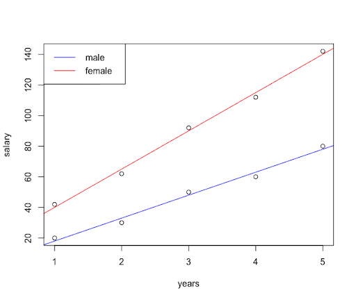
We can also plot the regression lines for both treatments.
plot(years,salary)
abline(lm(salary~years,data=subset(salary_data,gender=="m")),col="red")
abline(lm(salary~years,data=subset(salary_data,gender=="f")),col="blue")
legend("topleft",legend = c("male","female"),col=c("blue","red"),lty=1)
Finally, we can find the differences in the treatment LS means for various years (1, 3, and 5).
lsmeans_gender1 = emmeans::emmeans(aov1_unequal,pairwise~gender|years,at=list(years=1))
lsmeans_gender1$contrasts

lsmeans_gender3 = emmeans::emmeans(aov1_unequal,pairwise~gender|years,at=list(years=3))
lsmeans_gender3$contrasts

lsmeans_gender5 = emmeans::emmeans(aov1_unequal,pairwise~gender|years,at=list(years=5))
lsmeans_gender5$contrasts
years = 1:
 contrast estimate   SE df t.ratio p.value
 f - m         -22 3.46  6  -6.351  0.0007

years = 3:
 contrast estimate SE df t.ratio p.value
 f - m         -42  2  6 -21.000  <.0001

years = 5:
 contrast estimate   SE df t.ratio p.value
 f - m         -62 3.46  6 -17.898  <.0001