10: ANCOVA Part II
10: ANCOVA Part IIOverview
In this lesson, we will extend our ANCOVA to model quantitative predictors with higher-order polynomials by utilizing orthogonal polynomial coding. Fitting a polynomial to express the impact of the quantitative predictor on the response is also called trend analysis, and helps to evaluate the separate contributions of linear and nonlinear components of the polynomial. The examples discussed will illustrate how software can be used to fit higher-order polynomials within an ANCOVA model.
Objectives
- Use ANCOVA to analyze experiments that require polynomial modeling for quantitative predictors.
- Test hypotheses for treatment effects on polynomial coefficients.
10.1 - ANCOVA with Quantitative Factor Levels
10.1 - ANCOVA with Quantitative Factor LevelsAn Extended Overview of ANCOVA
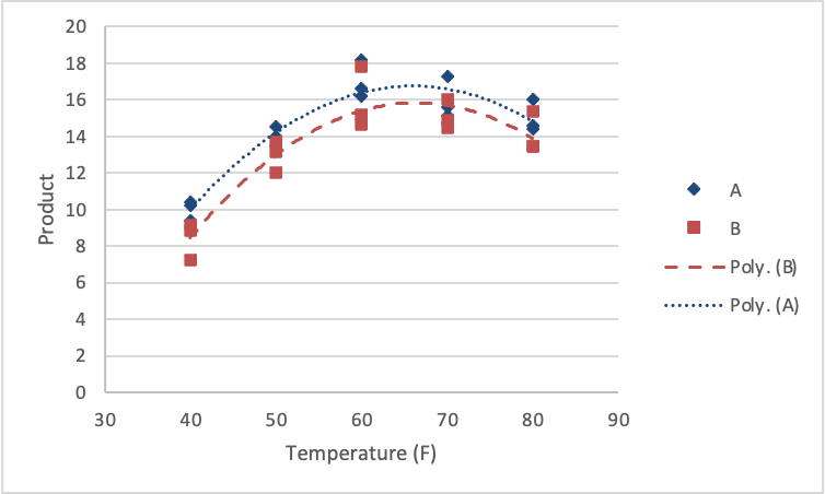
Designed experiments often contain treatment levels that have been set with increasing numerical values. For example, consider a chemical process which is hypothesized to vary by two factors: the Reagent type (A or B), and temperature. Researchers conducted an experiment that investigates a response at 40, 50, 60, 70, and 80 degrees (F) for each of the Reagent types.
You can find the data at QuantFactorData.csv
If temperature is considered as a categorical factor, we can proceed as usual with a 2 × 5 factorial ANOVA to evaluate the null hypotheses
\(H_0 \colon \mu_A = \mu_B\)
\(H_0 \colon \mu_{40} = \mu_{50} = \mu_{60} = \mu_{70} = \mu_{80}\)
and
\(H_0\colon\) no interaction.
Although the above hypotheses compare the response means for the process carried out at different temperatures, no conclusion can be made about the trend of the response as the temperature is increased.
In general, the trend effects of a continuous predictor are modeled using a polynomial where its non-constant terms represent the different trends, such as linear, quadratic, and cubic effects. These non-constant terms in the polynomial are called trend terms.
The statistical significance of these trend terms can be tested in an ANCOVA by adding columns into the design matrix (X) of the General Linear Model (see Lesson 4 for the definition of a design matrix). These additional columns will represent the trend terms and their interaction effects with the categorical factor. Inclusion of the trend term columns will facilitate significance testing for the overall trend effects, whereas the columns representing the interactions can be utilized to compare differences of each trend effect among the categorical factor levels.
In the chemical process example, if the quantitative property of temperature is used, we can carry out an ANCOVA by fitting a polynomial regression model to express the impact of temperature on the response. If a quadratic polynomial is desired, the appropriate ANCOVA design matrix can be obtained by adding two columns representing \(temp\) and \(temp^2\) to the existing column of ones representing the reagent type A (the reference category) and the dummy variable column representing the reagent type B.
The \(temp\) and \(temp^2\) terms allow us to investigate the linear and quadratic trends, respectively. Furthermore, the inclusion of columns representing the interactions between the reagent type and the two trend terms will facilitate the testing of differences between these two trends between the two reagent types. Note also that additional columns can be added appropriately to fit a polynomial of an even higher order.
Rule: To fit a polynomial of degree n, the response should be measured at least (n+1) distinct levels of the covariate. Preliminary graphics such as scatterplots are useful in deciding the degree of the polynomial to be fitted.
Suggestion: To reduce structural multicollinearity, centering the covariate by subtracting the mean is recommended. For more details see STAT 501 - Lesson 12: Multicollinearity
Using Technology
In SAS, this process would look like this:
/*centering the covariate creating x^2 */
                data centered_quant_factor;
                set quant_factor;
                x = temp-60;
                x2 = x**2;
                run;
                proc mixed data=centered_quant_factor method=type1;
                class reagent;
                model product=reagent x x2 reagent*x reagent*x2;
                title 'Centered';
                run;
Notice that we specify reagent as a class variable, but \(x\) and \(x^2\) enter the model as continuous variables. Also notice we use the Type I SS because the continuous variables show be considered in the model hierarchically. The regression coefficient of \(x\) and \(x^2\) can be used to test the significance of the linear and quadratic trends for reagent type A. The reference category and the interaction term coefficients can be used if these trends differ by categorical factor level. For example, testing the null hypothesis \(H_0 \colon \beta_{Reagent*x} = 0\) where \(\beta_{Reagent*x}\) is the regression coefficient of the \(Reagent*x\) term is equivalent to testing that the linear effects are the same for reagent type A and B.
SAS output:
Type 1 Analysis of Variance | ||||||||
|---|---|---|---|---|---|---|---|---|
Source | DF | Sum of Squares | Mean Square | Expected Mean Square | Error Term | Error DF | F Value | Pr > F |
reagent | 1 | 9.239307 | 9.239307 | Var(Residual) + Q(reagent,x2*reagent) | MS(Residual) | 24 | 8.95 | 0.0063 |
x | 1 | 97.600495 | 97.600495 | Var(Residual) + Q(x,x*reagent) | MS(Residual) | 24 | 94.52 | <.0001 |
x2 | 1 | 88.832986 | 88.832986 | Var(Residual) + Q(x2,x2*reagent) | MS(Residual) | 24 | 86.03 | <.0001 |
x*reagent | 1 | 0.341215 | 0.341215 | Var(Residual) + Q(x*reagent) | MS(Residual) | 24 | 0.33 | 0.5707 |
x2*reagent | 1 | 0.067586 | 0.067586 | Var(Residual) + Q(x2*reagent) | MS(Residual) | 24 | 0.07 | 0.8003 |
Residual | 24 | 24.782417 | 1.032601 | Var(Residual) | . | . | . | . |
The linear and quadratic effects were significant in describing the trend in the response. Further, the linear and quadratic effects are the same for each of the reagent types (no interactions). A figure of the results would look as follows.
First, we load and attach the Quant Factor data.
setwd("~/path-to-folder/")
                    QuantFactor_data <- read.csv("QuantFactorData.csv",header=T)
                    attach(QuantFactor_data)
Next, we center and square the response variable and augment the dataset with the new variables.
temp_center = temp-60
                    temp_center2 = temp_center^2
                    new_data = data.frame(QuantFactor_data,temp_center,temp_center2)
                    detach(QuantFactor_data); attach(new_data)
We can then fit the ANCOVA using the recentered data and obtain the Type 1 ANOVA table (because polynomial models are built hierarchically). The output suggests that the regression coefficients of both the linear and quadratic terms are not statistically different for the treatment levels, i.e. the interactions are not significant, therefore those terms would be removed (sequentially) from the final model.
lm1 = lm(product ~ reagent + temp_center + temp_center2 + reagent:temp_center + reagent:temp_center2)
                    aov1 = aov(lm1)
                    summary(aov1)
Df Sum Sq Mean Sq F value Pr(>F)
reagent 1 9.24 9.24 8.948 0.00634 **
temp_center 1 97.60 97.60 94.519 8.50e-10 ***
temp_center2 1 88.83 88.83 86.028 2.09e-09 ***
reagent:temp_center 1 0.34 0.34 0.330 0.57075
reagent:temp_center2 1 0.07 0.07 0.065 0.80026
Residuals 24 24.78 1.03
---
Signif. codes: 0 ‘***’ 0.001 ‘**’ 0.01 ‘*’ 0.05 ‘.’ 0.1 ‘ ’ 1The regression curve for reagent A and reagent B can be plotted with the following commands.
data_subsetA = subset(new_data,reagent=="A")
                    data_subsetB = subset(new_data,reagent=="B")
                    lmA = lm(product ~ temp_center + temp_center2, data = data_subsetA)
                    lmB = lm(product ~ temp_center + temp_center2, data = data_subsetB)
                    plot(temp,product,ylim=c(0,20),xlab="Temperature", ylab="Product",pch=ifelse(reagent=="A",23,22), col=ifelse(reagent=="A","blue","red"), lwd=2)
                    lines(data_subsetA$temp,fitted(lmA), col = "blue")
                    lines(data_subsetB$temp,fitted(lmB), col = "red")
                    legend("bottomright",legend=c("A","B"),pch=c(23,22),col=c("blue","red"))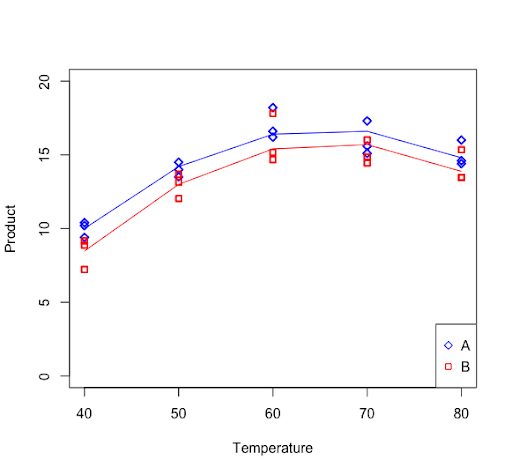
10.2 - Quantitative Predictors: Orthogonal Polynomials
10.2 - Quantitative Predictors: Orthogonal PolynomialsPolynomial trends in the response with respect to a quantitative predictor can be evaluated by using orthogonal polynomial contrasts, a special set of linear contrasts. This is an alternative to the regression analysis illustrated in the previous section, which may be affected by multicollinearity. Note that centering to remedy multicollinearity is effective only for quadratic polynomials. Therefore this simple technique of trend analysis performed via orthogonal polynomial coding will prove to be beneficial for higher-order polynomials. Orthogonal polynomials have the property that the cross-products defined by the numerical coefficients of their terms add to zero.
The orthogonal polynomial coding can be applied only when the levels of quantitative predictor are equally spaced. The method partitions the quantitative factor in the ANOVA table into independent single degrees of freedom comparisons. The comparisons are called orthogonal polynomial contrasts or comparisons.
Orthogonal polynomials are equations such that each is associated with a power of the independent variable (e.g. \(x\), linear; \(x^2\), quadratic; \(x^3\), cubic, etc.) In other words, orthogonal polynomials are coded forms of simple polynomials. The number of possible comparisons is equal to \(k-1\), where \(k\) is the number of quantitative factor levels. For example, if \(k=3\), only two comparisons are possible allowing for testing of linear and quadratic effects.
Using orthogonal polynomials to fit the desired model to the data allows us to eliminate collinearity while obtaining the same information as with simple polynomials.
A typical polynomial model of order \(k-1\) would be:
\(y = \beta_0 + \beta_1 x + \beta_2 x^2 + \cdots + \beta_{(k-1)} x^{(k-1)} + \epsilon\)
The simple polynomials used are \(x, x^2, \dots, x^{(k-1)}\). We can obtain orthogonal polynomials as linear combinations of these simple polynomials. If the levels of the predictor variable, \(x\) are equally spaced then one can easily use coefficient tables to determine the orthogonal polynomial coefficients that can be used to set up an orthogonal polynomial model.
If we are to fit the \((k-1)^{th}\) order polynomial using orthogonal contrasts coefficients, the general equation can be written as
\(y_{ij} = \alpha_0 + \alpha_1 g_{1i}(x) + \alpha_2 g_{2i}(x) + \cdots + \alpha_{(k-1)} g_{(k-1)i}(x)+\epsilon_{ij}\)
where \(g_{pi}(x)\) is a polynomial in \(x\) of degree \(p\) for the \(i^{th}\) level treatment factor. The parameter \(\alpha_p\) will depend on the coefficients \(\beta_p\). Using the properties of the function \(g_{pi}(x)\), one can show that the first five orthogonal polynomial are of the following form:
Mean: \(g_0(x)=1\)
Linear: \(g_1(x)=\lambda_1 \left( \dfrac{x-\bar{x}}{d}\right)\)
Quadratic: \(g_2(x)=\lambda_2 \left( \left(\dfrac{x-\bar{x}}{d}\right)^2-\left( \dfrac{t^2-1}{12} \right)\right)\)
Cubic: \(g_3(x)=\lambda_3 \left( \left(\dfrac{x-\bar{x}}{d}\right)^3- \left(\dfrac{x-\bar{x}}{d}\right)\left( \dfrac{3t^2-7}{20} \right)\right)\)
Quartic: \(g_4(x) = \lambda_4 \left( \left( \dfrac{x - \bar{x}}{d} \right)^4 - \left( \dfrac{x - \bar{x}}{d} \right)^2 \left( \dfrac{3t^2 - 13}{14} \right)+ \dfrac{3 \left(t^2 - 1\right) \left(t^2 - 9 \right)}{560} \right)\)
where \(t\) = number of levels of the factor, \(x\) = value of the factor level, \(\bar{x}\) = mean of the factor levels, and \(d\) = distance between factor levels.
In the next section, we will illustrate how the orthogonal polynomial contrast coefficients are generated, and the Factor SS is partitioned. This method will be required to fit polynomial regression models with terms greater than the quadratic because even after centering there will still be multicollinearity between \(x\) and \(x^3\) as well as between \(x^2\) and \(x^4\).
10.3 - Orthongonal Polynomials: Fungus Example
10.3 - Orthongonal Polynomials: Fungus ExampleFungus Example
Consider a treatment design consisting of five humidity level percentages (30, 40, 50, 60, and 70). Each of the five treatments is assigned randomly to three climate-controlled grow rooms in a completely randomized experimental design. The resulting fungus crop yields (lbs) are shown in the table below (Fungus Data):
Means (\(\bar{y}_i\)) | Humidity (x) | ||||
|---|---|---|---|---|---|
30 | 40 | 50 | 60 | 70 | |
13.1 | 17.1 | 19.5 | 18.7 | 18.9 | |
12.3 | 16.6 | 21.1 | 20.1 | 17.3 | |
13.3 | 17.4 | 19.3 | 18.2 | 17.5 | |
12.90 | 17.03 | 19.97 | 19.00 | 17.90 | |
We can see that the factor humidity has levels that are equally spaced. Therefore, we can use the orthogonal contrast coefficients to fit a polynomial to the response, fungus yields. With \(k=5\) levels, we can only fit up to a quartic term. The orthogonal polynomial contrast coefficients for the example are shown in Table 10.1. Here, \(r=3\) denotes the number of replicates, \(p=1,\dots,4\) denotes the term order, and \(i = 1,\dots,5\) denotes the factor level.
Humidity(x) | \(\bar{y}_i\) | Orthogonal Polynomial Coefficients \((g_{pi})\) | ||||
|---|---|---|---|---|---|---|
Mean | Linear | Quadratic | Cubic | Quartic | ||
30 | 12.90 | 1 | -2 | 2 | -1 | 1 |
40 | 17.03 | 1 | -1 | -1 | 2 | -4 |
50 | 19.97 | 1 | 0 | -2 | 0 | 6 |
60 | 19.00 | 1 | 1 | -1 | -2 | -4 |
70 | 17.90 | 1 | 2 | 2 | 1 | 1 |
\(\lambda_p\) | - | 1 | 1 | 5/6 | 35/12 | |
Sum = \(\sum g_{pi}\bar{y}_{i.}\) | 86.80 | 11.97 | -14.37 | 1.07 | 6.47 | |
Divisor = \(\sum g_{pi}^{2}\) | 5 | 10 | 14 | 10 | 70 | |
\(SSP_p=r(\sum g_{pi}\bar{y}_{i.})^2/\sum g_{pi}^{2}\) | - | 42.96 | 44.23 | 0.34 | 1.79 | |
\(\hat{\alpha}_p=\sum g_{pi}\bar{y}_{i.}/\sum g_{pi}^{2}\) | 17.36 | 1.20 | -1.03 | 0.11 | 0.09 | |
As mentioned before, one can easily find the orthogonal polynomial coefficients \((g_{pi})\) for a different order of polynomials using pre-documented tables for equally spaced intervals. However, let us try to understand how the coefficients are obtained.
First note that the five values of \(x\) are 30, 40, 50, 60, and 70. Therefore, \(\bar{x} = 50\) and the spacing \(d = 10\). This means that the five values of \(\dfrac{x - \bar{x}}{d}\) are -2, -1, 0, 1, and 2.
Linear coefficients:
Using the linear orthogonal polynomial formula seen in Section 10.2, the polynomial \(g_{1i}\) for linear coefficients can be calculated as follows.
Linear Coefficient Polynomials | |||||
|---|---|---|---|---|---|
\(x\) | 30 | 40 | 50 | 60 | 70 |
\((x-50)\) | -20 | -10 | 0 | 10 | 20 |
\(\frac{(x-50)}{10}\) | -2 | -1 | 0 | 1 | 2 |
Linear orthogonal polynomial | \((-2)\lambda_1\) | \((-1)\lambda_1\) | \((0)\lambda_1\) | \((1)\lambda_1\) | \((2)\lambda_1\) |
To obtain the final set of coefficients we choose \(\lambda_1\) so that the coefficients are integers. Therefore, we set \(\lambda_1 = 1\) and obtain the coefficient values \((g_{1i})\) seen in the "Linear" column of Table 10.1.
Quadratic coefficients:
Using the quadratic orthogonal polynomial formula seen in Section 10.2, the polynomial \(g_{2i}\) for linear coefficients turns out to be:
\(\begin{align*}
&\left( (-2)^2 - \left( \dfrac{5^2 - 1}{12}\right)\right)\lambda_2,
\left( (-1)^2 - \left( \dfrac{5^2 - 1}{12}\right)\right)\lambda_2,
\\& \left( (0)^2 - \left( \dfrac{5^2 - 1}{12}\right)\right)\lambda_2,
\left( (1)^2 - \left( \dfrac{5^2 - 1}{12}\right)\right)\lambda_2,
\\& \left( (2)^2 - \left( \dfrac{5^2 - 1}{12}\right)\right)\lambda_2
\end{align*}\)
which simplified gives:
\((2)\lambda_2, (-1)\lambda_2, (-2)\lambda_2, (-1)\lambda_2, (2)\lambda_2\)
To obtain the final set of coefficients we choose \(\lambda_2\) so that the coefficients are integers. Therefore, we set \(\lambda_2 = 1\) and obtain the coefficient values \((g_{2i})\) seen in the "Quadratic" column of Table 10.1.
Cubic coefficients:
The polynomial \(g_{3i}\) for cubic coefficients turns out to be:
\(\begin{align*}
&\left( (-2)^3 - (-2) \left( \dfrac{3(5^2) - 7}{20} \right)\right)\lambda_3,
\left( (-1)^3 - (-1) \left( \dfrac{3(5^2) - 7}{20} \right)\right)\lambda_3,
\\& \left( (0)^3 - (0) \left( \dfrac{3(5^2) - 7}{20} \right)\right)\lambda_3,
\left( (1)^3 - (1) \left( \dfrac{3(5^2) - 7}{20} \right)\right)\lambda_3,
\\& \left( (2)^3 - (2) \left( \dfrac{3(5^2) - 7}{20} \right)\right)\lambda_3
\end{align*}\)
which simplified gives:
\((-\dfrac{6}{5})\lambda_3, (\dfrac{12}{5})\lambda_3, (0)\lambda_3, (\dfrac{-12}{5})\lambda_3, (\dfrac{6}{5})\lambda_3\)
To obtain the final set of coefficients we choose \(\lambda_3\) so that the coefficients are integers. Therefore, we set \(\lambda_3 = 5/6\) and obtain the coefficient values \((g_{3i})\) seen in the "Cubic" column of Table 10.1.
Quartic coefficients:
The polynomial \(g_{4i}\) can be used to obtain the quartic coefficients in the same way as above.
Each set of coefficients corresponds to a contrast among the treatments. Notice the sum of coefficients is equal to zero (e.g. the quartic coefficients \((1, -4, 6, -4, 1)\) sum to zero, etc). Using orthogonal polynomial contrasts, we can partition the treatment sums of squares into a set of additive sums of squares corresponding to orthogonal polynomial contrasts. The contrast computations are identical to those we learned in Lesson 2.5. The resulting partitions can be used to sequentially test the significance of the linear, quadratic, cubic, and quartic terms in the model and find the polynomial order appropriate for the data.
Table 10.1 shows how to obtain the sums of squares for each component \( (SSP_p) \) and compute the estimates of the \(\alpha_p\) coefficients for the orthogonal polynomial equation. Using the results in Table 10.1, we have estimated the orthogonal polynomial equation as:
\(\hat{y}_i = 17.36 + 1.20 g_{1i} - 1.03 g_{2i} + 0.11 g_{3i} + 0.09g_{4i}\)
Table 10.2 summarizes how the treatment sums of squares are partitioned and their test results.
Source of Variation | Degrees of Freedom | Sum of Squares | Mean Square | F | Pr > F |
|---|---|---|---|---|---|
Density | 4 | 89.32 | 22.331 | 35.48 | 0.000 |
Error | 10 | 6.29 | 0.629 |
Contrast | DF | Contrast SS | Mean Square | F | Pr > F |
|---|---|---|---|---|---|
Linear | 1 | 42.96 | 42.96 | 68.26 | 0.000 |
Quadratic | 1 | 44.23 | 44.23 | 70.28 | 0.000 |
Cubic | 1 | 0.34 | 0.34 | 0.54 | 0.478 |
Quartic | 1 | 1.79 | 1.79 | 2.85 | 0.122 |
To test whether any of the polynomials are significant (i.e. \(H_0: \alpha_1 = \alpha_2 = \alpha_3 = \alpha_4 = 0\)), we can use the global F-test where the test statistic is equal to 35.48. We see that the p-value is almost zero and therefore we can conclude that at the 5% level, at least one of the polynomials is significant. Using the orthogonal polynomial contrasts we can determine which of the polynomials are useful. Table 10.2 shows that for this example only the linear and quadratic terms are useful. Removing the insignificant terms, the estimated orthogonal polynomial equation becomes:
\(\hat{y}_i = 17.36 + 1.20 g_{1i} - 1.03 g_{2i}\)
The polynomial relationship expressed as a function of y and x in actual units of the observed variables is more informative than when expressed in units of the orthogonal polynomial.
We can obtain the polynomial relationship using the actual units of observed variables by back-transforming using the formulas seen in Section 10.2. The necessary quantities to back-transform are \(\lambda_1=\lambda_2=1, d=10, \bar{x}=50\) and t = 5. Substituting these values we obtain
\(\begin{align}
\hat{y}&=17.36+1.20g_{1i}-1.03g_{2i}\\
&=17.36+1.20(1)\left( \dfrac{x-50}{10} \right)-1.03(1)\left( \left( \dfrac{x-50}{10} \right)^2-\dfrac{5^2-1}{12} \right)\\
\end{align}\)
which simplifies to
\(\hat{y}=-12.23+1.15x-0.01x^2\)
Using Technology
Below is the code for generating polynomials from the IML procedure in SAS:
/* read the fungus data set*/
/* Generating Ortho_Polynomials from IML */
proc iml;
  x={30 40 50 60 70};
  xpoly=orpol(x,4); /* the '4' is the df for the quantitative factor */
  humidity=x`; new=humidity || xpoly;
  create out1 from new[colname={"humidity" "xp0" "xp1" "xp2" "xp3" "xp4"}];
  append from new; close out1;
quit;
proc print data=out1;
run;

/* Here data is sorted and then merged with the original dataset */
proc sort data=fungal;
  by humidity;
run;
data ortho_poly; merge out1 fungal;
  by humidity;
run;
proc print data=ortho_poly;
run;

/* The following code will then generate the results shown in the
	notes*/
proc mixed data=ortho_poly method=type1;
  class;
  model yield=xp1 xp2 xp3 xp4/ solution;
  title 'Using Orthog polynomials from IML';
  ods select SolutionF;
run;

/*We can use proc glm to obtain the same results without using
   IML codings. Proc glm will use the orthogonal contrast coefficients directly*/
proc glm data=fungal;
 class humidity;
 model yield = humidity;
 contrast 'linear' humidity -2 -1 0 1 2;
 contrast 'quadratic' humidity 2 -1 -2 -1 2;
 contrast 'cubic' humidity -1 2 0 -2 1;
 contrast 'quatic' humidity 1 -4 6 -4 1;
 lsmeans humidity;
run;
Analysis of Variance | ||||||||
|---|---|---|---|---|---|---|---|---|
Source | DF | Sum of Squares | Mean Square | ExpectedMean Square | Error Term | Error DF | F Value | Pr > F |
xp1 | 1 | 43.200000 | 43.200000 | Var(Residual) + Q(xp1) | MS(Residual) | 10 | 57.75 | < .0001 |
xp2 | 1 | 42.000000 | 42.000000 | Var(Residual) + Q(xp2) | MS(Residual) | 10 | 56.15 | < .0001 |
xp3 | 1 | 0.300000 | 0.300000 | Var(Residual) + Q(xp2) | MS(Residual) | 10 | 0.40 | 0.5407 |
xp4 | 1 | 2.100000 | 2.100000 | Var(Residual) + Q(xp4) | MS(Residual) | 10 | 2.81 | 0.1248 |
Residual | 10 | 7.480000 | 7.480000 | Var(Residual) | ||||
Fitting a Quadratic Model with Proc Mixed
Often we can see that only a quadratic curvature is of interest in a set of data. In this case, we can plan to simply run an order 2 (quadratic) polynomial and can easily use proc mixed (the general linear model). This method requires centering the quantitative variable levels by subtracting the mean of the levels (50) and then creating the quadratic polynomial terms.
data fungal;
  set fungal;
  x=humidity-50;
  x2=x**2;
run;
proc mixed data=fungal method=type1;
  class;
  model yield = x x2;
run;
The output is:
Type 1 Analysis of Variance | ||||||||
|---|---|---|---|---|---|---|---|---|
Source | DF | Sum of Squares | Mean Square | Expected Mean Square | Error Term | Error DF | F Value | Pr > F |
x | 1 | 42.960333 | 42.960333 | Var(Residual) + Q(x) | MS(residual) | 12 | 61.18 | <.0001 |
x2 | 1 | 44.228810 | 44.228810 | Var(Residual) + Q(x2) | MS(residual) | 12 | 62.98 | <.0001 |
Residual | 12 | 8.426857 | 0.702238 | Var(Residual) | ||||
We can also generate the solutions (coefficients) for the model with the following code
proc mixed data=fungal method=type1;
  class;
  model yield = x x2 / solution;
run;
which gives the following output for the regression coefficients.
Solution for Fixed Effects | |||||
|---|---|---|---|---|---|
Effect | Estimate | Standard Error | DF | t Value | Pr > |t| |
Intercept | 19.4124 | 0.3372 | 12 | 57.57 | <.0001 |
x | 0.1197 | 0.01530 | 12 | 7.82 | <.0001 |
x2 | -0.01026 | 0.001293 | 12 | -7.94 | <.0001 |
Here we need to remember that the regression was based on centered values for the predictor, so we have to back-transform to get the coefficients in terms of the original variables. For example, the fitted second-order model for one predictor variable that is expressed in terms of centered values \(x = X-\bar{X}\):
\(\hat{Y}=b_0+b_1x+b_{2}x^2\)
becomes in terms of the original X variable:
\(\hat{Y}=b'_0+b'_1X+b'_{2}X^2\)
where:
\(\begin{align}
b'_0&=b_0-b_1\bar{X}+b_{2}\bar{X}^2\\
b'_1&=b_1-2b_{2}\bar{X}\\
b'_{2}&=b_{2}\\
\end{align}\)
In the example above, this back-transformation uses the estimates from the Solutions for Fixed Effects table as follows.
data backtransform;
  bprime0=19.4124-(0.1197*50)+(-0.01026*(50**2));
  bprime1=0.1197-(2*-0.01026*50);
  bprime2=-0.01026;
  title 'bprime0=b0-(b1*meanX)+(b2*(meanX)2)';
  title2 'bprime1=b1-2*b2*meanX';
  title3 'bprime2=b2';
run;
proc print data=backtransform;
 var bprime0 bprime1 bprime2;
run;
The output is then:
Obs | bprime0 | bprime1 | bprime2 |
|---|---|---|---|
1 | -12.2226 | 1.1457 | -0.01026 |
First, load and attach the Fungus data.
setwd("~/path-to-folder/")
fungal_data <- read.table("fungus_data.txt",header=T)
attach(fungal_data)
R has a built-in function for generating orthogonal polynomials which we utilize to obtain the Type 1 ANOVA table.
poly_lm = lm(yield ~ poly(humidity,4))
poly_aov1 = aov(poly_lm)
summary(poly_aov1)
Df Sum Sq Mean Sq F value Pr(>F) poly(humidity, 4) 4 89.32 22.331 35.48 7e-06 *** Residuals 10 6.29 0.629 --- Signif. codes: 0 ‘***’ 0.001 ‘**’ 0.01 ‘*’ 0.05 ‘.’ 0.1 ‘ ’ 1
It is clear from the F-test that at least one of the polynomial terms is significant. We can examine the t-tests of the individual terms using the summary function.
summary(poly_lm)Call: lm(formula = yield ~ poly(humidity, 4))
Residuals:
    Min      1Q  Median      3Q     Max
-0.8000 -0.5333 -0.3000  0.3833  1.1333
Coefficients:
Estimate Std. Error t value Pr(>|t|)
(Intercept) 17.3600 0.2048 84.753 1.28e-15 ***
poly(humidity, 4)1 6.5544 0.7933 8.262 8.87e-06 ***
poly(humidity, 4)2 -6.6505 0.7933 -8.383 7.80e-06 ***
poly(humidity, 4)3 0.5842 0.7933 0.736 0.478
poly(humidity, 4)4 1.3387 0.7933 1.688 0.122
---
Signif. codes: 0 ‘***’ 0.001 ‘**’ 0.01 ‘*’ 0.05 ‘.’ 0.1 ‘ ’ 1Residual standard error: 0.7933 on 10 degrees of freedom Multiple R-squared: 0.9342, Adjusted R-squared: 0.9079 F-statistic: 35.48 on 4 and 10 DF, p-value: 7.005e-06
As is commonly found, only the quadratic curvature is of interest. We can then fit a standard quadratic model, first recentering the response as seen in previous sections.
humidity_center = humidity-50
humidity_center2 = humidity_center^2
new_data = data.frame(fungal_data,humidity_center,humidity_center2)
detach(fungal_data); attach(new_data)

quad_lm = lm(yield ~ humidity_center + humidity_center2)
aov1_quad = aov(quad_lm)
summary(aov1_quad)
Df Sum Sq Mean Sq F value Pr(>F) humidity_center 1 42.96 42.96 61.18 4.73e-06 *** humidity_center2 1 44.23 44.23 62.98 4.08e-06 *** Residuals 12 8.43 0.70 --- Signif. codes: 0 ‘***’ 0.001 ‘**’ 0.01 ‘*’ 0.05 ‘.’ 0.1 ‘ ’ 1
The following coefficients are produced.
quad_lm$coefficients (Intercept) humidity_center humidity_center2
19.4123810 0.1196667 -0.0102619 To obtain the coefficients in terms of the original variables, we can back-transform these coefficients (output not shown).
b_0_prime = 19.4123810-0.1196667*50-0.0102619*50^2
b_0_prime
b_1_prime = 0.1196667-0.0102619*(-2*50)
b_1_prime
b_2_prime = -0.0102619
b_2_prime
10.4 - Lesson 10 Summary
10.4 - Lesson 10 SummaryThe versatility of the ANCOVA model has been illustrated in Lessons 9 and 10. In application, it is often used in ANOVA settings to adjust or 'control for' a covariate that may be masking real treatment differences. In regression settings, researchers may be focused on a family of regression relationships, and are interested in testing for significant differences among regression coefficients across different groups. These approaches are like two sides of the same coin.
In terms of model development, ANOVA and regression approaches converge in the general linear model as ANCOVA. Mastery of ANCOVA methodology is arguably one of the most important tools to have in an applied statistician's toolbox.