12: Cross-over Repeated Measure Designs
12: Cross-over Repeated Measure DesignsOverview
In this lesson, we will be discussing the basics of cross-over repeated measure designs. A cross-over design is a repeated measures design in which each experimental unit is given each of the different treatment levels over the course of the experiment. This means that over time each experimental unit is assigned to a specific ordered sequence of different treatment levels. This is in contrast to a repeated measures design in time, discussed in the previous lesson, where multiple measurements from the same experimental unit assigned to a specific treatment level are taken through time.
Objectives
- Recognize a cross-over repeated measures design.
- Understand what a wash-out period is.
- Test for the significance of carry-over effects.
- Adjust treatment means to account for carry-over effects.
12.1 - Introduction to Cross-over Designs
12.1 - Introduction to Cross-over DesignsThe simplest cross-over design is a 2-level treatment, 2-period design. If we use A and B to represent the two treatment levels, then we can build the following table to represent their administering sequences.
| Sequence | Period 1 | Period 2 |
|---|---|---|
| 1 | A | B |
| 2 | B | A |
Experimental units are randomly assigned to receive one of the two different sequences. For example, if this were a clinical trial, patients assigned to sequence 2 would be given treatment B first, then after assessment of their condition, given treatment A and their condition re-assessed.
The complicated part of the cross-over design is the potential for carry-over effects. A carry-over effect is when the response to a particular treatment level has been influenced by the previous application of a different treatment level.
The presence of carry-over effects is dealt with differently by different researchers. Having a sufficiently long wash-out period is one way to reduce carry-over effects. A wash-out period is a gap in time between the application of the treatment levels such that any residual effect of a previous treatment level has been dissipated and there is no detectable carry-over effect.
However, there may be instances where significant carry-over effects may exist and sufficiently long wash-out periods may not be practically feasible. In such situations, an adjustment for carry-over effects would be appropriate during the statistical analysis.
If the treatment has only 2 levels, it is sufficient to simply include a ‘sequence’ categorical variable in the model to assess the presence of a carry-over effect. If the sequence variable is significant, then a detectable carry-over effect exists. However, with more than two treatment levels, the complexity of the analysis rises sharply. For 3 levels of treatment, 3 periods will be needed, and now we have 3! = 6 sequences to consider. What is needed in this case, in addition to a sequence variable, is a way to adjust the assessment of treatment effects for the presence of carry-over effects. This can be accomplished with a set of coded covariates in a repeated-measures ANCOVA.
12.2 - Coding for Carry-over Covariates: Psychiatry Example
12.2 - Coding for Carry-over Covariates: Psychiatry ExampleLate Dr. Steve Arnold (Penn State), came up with a satisfactory solution to account for carry-over effects in the data analysis. The following example will illustrate how the procedure works.
Psychiatrists want to evaluate the effect of three drugs on severe post-traumatic stress disorder (PTSD) symptoms. The three drugs are administered to each patient in a sequence over three periods. The change in each patient's functional capability score (FCS) from baseline is recorded at the end of each period. A total of six sequences were used and two patients were assigned to each sequence of treatments.
The cross-over design can be summarized as:
Period | |||
|---|---|---|---|
Sequence | 1 | 2 | 3 |
1 | A | B | C |
2 | B | C | A |
3 | C | A | B |
4 | A | C | B |
5 | B | A | C |
6 | C | B | A |
If we look at the first part of the dataset (Psychiatry Data), we can see the following:
PER | SEQ | DRUG | PAT | FCS |
|---|---|---|---|---|
1 | 1 | A | 1 | 41 |
1 | 1 | A | 2 | 46 |
1 | 2 | B | 1 | 35 |
1 | 2 | B | 2 | 42 |
1 | 3 | C | 1 | 46 |
1 | 3 | C | 2 | 52 |
1 | 4 | A | 1 | 65 |
1 | 4 | A | 2 | 69 |
1 | 5 | B | 1 | 61 |
1 | 5 | B | 2 | 66 |
1 | 6 | C | 1 | 52 |
1 | 6 | C | 2 | 37 |
2 | 1 | B | 1 | 52 |
2 | 1 | B | 2 | 54 |
2 | 2 | C | 1 | 33 |
2 | 2 | C | 2 | 36 |
2 | 3 | A | 1 | 46 |
2 | 3 | A | 2 | 47 |
2 | 4 | C | 1 | 39 |
We need now to add two columns to use an effect-type coding for the 3 treatment levels. We define the following coding:
A | \(x_1\) | \(x_2\) |
|---|---|---|
1 | 0 | |
B | 0 | 1 |
C | -1 | -1 |
Here \(x_1\) and \(x_2\) will be columns we create in the data to input for all of the rows of data. The coding values depend on which treatment level is administered during the previous period. For example, if treatment A was administered in the previous period, then coding values would be \(x_1=1, x_2=0\).
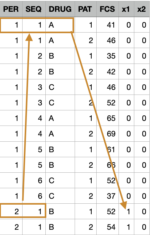
There will be no entries for the first period because on the first application of each treatment there are no treatments that have preceded it. Therefore a 0 is used as the coding value for both \(x_1\) and \(x_2\). The augmented dataset will be the following:
PER | SEQ | DRUG | PAT | FCS | x1 | x2 |
|---|---|---|---|---|---|---|
1 | 1 | A | 1 | 41 | 0 | 0 |
1 | 1 | A | 2 | 46 | 0 | 0 |
1 | 2 | B | 1 | 35 | 0 | 0 |
1 | 2 | B | 2 | 42 | 0 | 0 |
1 | 3 | C | 1 | 46 | 0 | 0 |
1 | 3 | C | 2 | 52 | 0 | 0 |
1 | 4 | A | 1 | 65 | 0 | 0 |
1 | 4 | A | 2 | 69 | 0 | 0 |
1 | 5 | B | 1 | 61 | 0 | 0 |
1 | 5 | B | 2 | 66 | 0 | 0 |
1 | 6 | C | 1 | 52 | 0 | 0 |
1 | 6 | C | 2 | 37 | 0 | 0 |
2 | 1 | B | 1 | 52 | 1 | 0 |
2 | 1 | B | 2 | 54 | 1 | 0 |
2 | 2 | C | 1 | 33 | 0 | 1 |
2 | 2 | C | 2 | 36 | 0 | 1 |
2 | 3 | A | 1 | 46 | -1 | -1 |
2 | 3 | A | 2 | 47 | -1 | -1 |
2 | 4 | C | 1 | 39 | 1 | 0 |
Looking at Period 2, sequence 1, treatment B, we can refer back to the Sequence chart and see that it was preceded by treatment level A, so we assign \(x_1 = 1\), and \(x_2 = 0\), indicating that it was treatment A that could produce a carry-over effect here.
The process can be repeated to define the coding variables for each entry in the dataset. The coded variables \(x_1\) and \(x_2\) are then entered into the general linear model as continuous covariates and LSmeans for treatments are adjusted for carry-over effects.
12.3 - Using Technology: Psychiatry Example
12.3 - Using Technology: Psychiatry ExampleSAS®
The SAS code given below will run a repeated measures ANCOVA in SAS for the psychiatry example from section 12.2.
data FCS;
infile datalines delimiter='09'x;
input per seq drug $ pat FCS x1 x2;
datalines;
1	1	A	1	41	0	0
1	1	A	2	46	0	0
1	2	B	1	35	0	0
1	2	B	2	42	0	0
1	3	C	1	46	0	0
1	3	C	2	52	0	0
1	4	A	1	65	0	0
1	4	A	2	69	0	0
1	5	B	1	61	0	0
1	5	B	2	66	0	0
1	6	C	1	52	0	0
1	6	C	2	37	0	0
2	1	B	1	52	1	0
2	1	B	2	54	1	0
2	2	C	1	33	0	1
2	2	C	2	36	0	1
2	3	A	1	46	-1	-1
2	3	A	2	47	-1	-1
2	4	C	1	39	1	0
2	4	C	2	42	1	0
2	5	A	1	48	0	1
2	5	A	2	50	0	1
2	6	B	1	47	-1	-1
2	6	B	2	49	-1	-1
3	1	C	1	44	0	1
3	1	C	2	48	0	1
3	2	A	1	48	-1	-1
3	2	A	2	50	-1	-1
3	3	B	1	38	1	0
3	3	B	2	41	1	0
3	4	B	1	42	-1	-1
3	4	B	2	45	-1	-1
3	5	C	1	42	1	0
3	5	C	2	46	1	0
3	6	A	1	49	0	1
3	6	A	2	52	0	1
;
run;

/*Obtaining fit Statistics*/
proc mixed data=FCS;
  class per seq drug pat;
  model FCS = per drug seq x1 x2/ddfm=kr;
  repeated per / subject=pat(seq) type=cs rcorr;
  ods output FitStatistics=FitCS (rename=(value=CS)) FitStatistics=FitCSp;
  title 'Compound Symmetry';
run;

proc mixed data=FCS;
  class per seq drug pat;
  model FCS = per drug seq x1 x2/ddfm=kr;
  repeated per / subject=pat(seq) type=AR(1) rcorr;
  ods output FitStatistics=FitAR1 (rename=(value=AR1)) FitStatistics=FitAR1p;
  title 'Autoregressive Lag 1';
run;

proc mixed data=FCS;
  class per seq drug pat;
  model FCS = per drug seq x1 x2/ddfm=kr;
  repeated per / subject=pat(seq) type=UN rcorr;
  ods output FitStatistics=FitUN (rename=(value=UN)) FitStatistics=FitUNp;
 title 'Unstructured';
run;

proc mixed data=FCS;
  class per seq drug pat;
  model FCS = per drug seq x1 x2/ddfm=kr;
  repeated per / subject=pat(seq) type=CSH rcorr;
  ods output FitStatistics=FitCSH (rename=(value=CSH)) FitStatistics=FitCSHp;
  title 'HETEROGENOUS COMPOUND SYMMETRY';
run;

data fits;
 merge FitCS FitAR1 FitUN FITCSH;
 by descr;
run;
ods listing; title 'Summerized Fit Statistics'; run;
proc print data=fits; run;

/* Model Adjusting for carryover effects */
proc mixed data= FCS;
  class per seq drug pat;
  model FCS = per drug seq x1 x2/ddfm=kr;
  repeated per / subject=pat(seq) type=UN;
  store out_FCS;
 run;

proc plm restore=out_FCS;
  lsmeans drug / adjust=tukey plot=meanplot cl lines;
  ods exclude diffs diffplot;
run;

/* Reduced Model, Ignoring carryover effects */
proc mixed data= FCS;
  class per seq drug pat;
  model FCS = per drug seq/ddfm=kr;
  repeated per / subject=pat(seq) type=UN;
  lsmeans drug / pdiff adjust=tukey;
run;
The results of the fit statistics are as follows:
| Obs | Descr | CS | AR1 | UN | CSH |
|---|---|---|---|---|---|
| 1 | -2 Res Log Likelihood | 184.1 | 186.7 | 148.1 | 155.6 |
| 2 | AIC (Smaller is Better) | 188.1 | 190.7 | 160.1 | 163.6 |
| 3 | AICC (Smaller is Better) | 188.7 | 191.3 | 165.0 | 165.7 |
| 4 | BIC (Smaller is Better) | 189.1 | 191.7 | 163.0 | 165.5 |
Notice we consider an additional covariance structure, CSH. The CSH covariance structure is similar to CS in that is also has a constant correlation in the off-diagonal elements. However, the diagonal elements (the variance at each time point) can be different.
Based on the fit statistic AIC (also AICC and BIC) the unstructured covariance structure (type=UN) is better compared to CS, CSH or AR(1).
Here is the output that is generated for the full model:
| Type 3 Tests of Fixed Effects | ||||
|---|---|---|---|---|
| Effect | Num DF | Den DF | F Value | Pr > F |
| per | 2 | 5.49 | 1.08 | 0.4027 |
| drug | 2 | 7.04 | 148.74 | <.0001 |
| seq | 5 | 6.79 | 5.37 | 0.0255 |
| x1 | 1 | 6.98 | 18.88 | 0.0034 |
| x2 | 1 | 6.98 | 83.96 | <.0001 |
The Type 3 tests shown above are 'model dependent' meaning that the sum of squares for each of the effects are adjusted for the other effects in the model. In this case, we have adjusted for the presence of carry-over effects. As the drug is significant, it is appropriate to generate LSmeans and the Tukey-Kramer mean comparisons for the drug factor.
| drug Least Squares Means | ||||||||
|---|---|---|---|---|---|---|---|---|
| DIET | Estimate | Standard Error | DF | t Value | Pr > |t| | Alpha | Lower | upper |
| A | 52.7336 | 1.3810 | 4.113 | 38.18 | < 0.0001 | 0.05 | 48.9404 | 56.5268 |
| B | 45.8350 | 1.3810 | 4.113 | 33.19 | < 0.0001 | 0.05 | 42.0418 | 49.6283 |
| C | 43.0980 | 1.3810 | 4.113 | 31.21 | < 0.0001 | 0.05 | 39.3048 | 46.8913 |
To see the adjustment on the treatment means, we can compare the LSmeans for a reduced model that does not contain the carry-over covariates.
| Full Model with Covariates | ||
|---|---|---|
| Effect | DIET | Estimate |
| DIET | A | 52.7336 |
| DIET | B | 45.8350 |
| DIET | C | 43.0980 |
| Reduced Model (without carry-over covariates) | ||
|---|---|---|
| Effect | DIET | Estimate |
| DIET | A | 52.1625 |
| DIET | B | 46.9760 |
| DIET | C | 42.5282 |
Although the differences in the LSmeans between the two models are small in this particular example, these carry-over effect adjustments can be very important in many research situations.
12.4 - Testing the Significance of the Carry-over Effect: Psychiatry Example
12.4 - Testing the Significance of the Carry-over Effect: Psychiatry ExampleTo test for the overall significance of carry-over effects, we can drop the carry-over covariates (\(x_1\) and \(x_2\) in our example) and re-run the ANOVA. Because the reduced model is a subset of the full model that includes the covariates, we can construct a likelihood ratio test.
\(\Delta G^2=(-2logL_{Reduced})-(-2logL_{Full})\)
with \(df_{Reduced}-df_{Full}\) degrees of freedom
The -2logL values are provided in the SAS Fit Statistics output for each model. For our example, the SAS output for the Full model with carry-over covariates is:
| Fit Statistics | |||||
|---|---|---|---|---|---|
| -2 Res Log Likelihood | 148.1 | ||||
| AIC (smaller is better) | 160.1 | ||||
| AICC (smaller is better) | 165.0 | ||||
| BIC (smaller is better) | 163.0 | ||||
And for the reduced model without the carry-over covariates is:
| Fit Statistics | |||||
|---|---|---|---|---|---|
| -2 Res Log Likelihood | 171.2 | ||||
| AIC (smaller is better) | 183.2 | ||||
| AICC (smaller is better) | 187.6 | ||||
| BIC (smaller is better) | 186.1 | ||||
So,
\(\Delta G^2 =171.2-148.1=23.1\)
and with
\(\chi^2_{0.05, 2}=5.991\)
we conclude that there are significant carry-over effects.
12.5 - Try it!
12.5 - Try it!Exercise 1: Memory Recall
Ginkgo Biloba is recognized as a herbal remedy for memory improvement. To investigate its effectiveness on memory recall, a cross-over study was planned using 3 treatments: one tablet of 120mg Ginkgo Biloba (G), one tablet of 200mg Caffeine pill (C), and sleep for 2 hours before the recall test (S). The assignment order of the 3 treatments to participants was determined by randomly assigning 12 college students (Id) to one of 6 possible sequences of the 3 treatments. The student recall capability was assessed based on a recall score (the higher the better) and the 3 treatments were given over 3 consecutive days. On each day, only one treatment was administered before one 1 hour of taking the recall test at 2pm.
Which variable signifies the experimental unit?
IdWhat is the washout period?
One dayHow many periods are required?
3How many replicates are there?
2Perform a statistical analysis to determine if the treatments vary with regard to memory recall. The data can be found in Cross_over_Ex1.txt
Using SAS...
DATA CROSS_OVER;
                INPUT score  Seq $ PER  Id  TRT $ X1  X2;
                DATALINES;
                74  CGS  1  1  C  0  0
                45  CGS  1  2  C  0  0
                92  CSG  1  3  C  0  0
                94  CSG  1  4  C  0  0
                79  GCS  1  5  G  0  0
                35  GCS  1  6  G  0  0
                31  GSC  1  7  G  0  0
                40  GSC  1  8  G  0  0
                106  SCG  1  9  S  0  0
                60  SCG  1  10  S  0  0
                80  SGC  1  11  S  0  0
                110  SGC  1  12  S  0  0
                41  CGS  2  1  G  1  0
                20  CGS  2  2  G  1  0
                50  CSG  2  3  S  1  0
                88  CSG  2  4  S  1  0
                92  GCS  2  5  C  0  1
                50  GCS  2  6  C  0  1
                32  GSC  2  7  S  0  1
                54  GSC  2  8  S  0  1
                120  SCG  2  9  C  -1  -1
                80  SCG  2  10  C  -1  -1
                75  SGC  2  11  G  -1  -1
                55  SGC  2  12  G  -1  -1
                64  CGS  3  1  S  0  1
                30  CGS  3  2  S  0  1
                55  CSG  3  3  G  -1  -1
                55  CSG  3  4  G  -1  -1
                76  GCS  3  5  S  1  0
                50  GCS  3  6  S  1  0
                38  GSC  3  7  C  -1  -1
                66  GSC  3  8  C  -1  -1
                85  SCG  3  9  G  1  0
                40  SCG  3  10  G  1  0
                88  SGC  3  11  C  0  1
                86  SGC  3  12  C  0  1
                ;
                RUN;

                proc mixed data=CROSS_OVER;
                  class PER TRT SEQ  ID;
                  model SCORE=PER  TRT SEQ  X1 X2 / ddfm=kr;
                  repeated PER /subject=ID(SEQ) type=cs rcorr;
                  ods output FitStatistics=FitCS (rename=(value=CS)) FitStatistics=FitCSp;
                  title 'Compound Symmetry';
                run;
                title ' '; run;
                proc mixed data=CROSS_OVER;
                  class PER TRT SEQ  ID;
                  model SCORE=PER  TRT SEQ  X1 X2 / ddfm=kr;
                  repeated PER /subject=ID(SEQ) type=AR(1) rcorr;
                  ods output FitStatistics=FitAR1 (rename=(value=AR1)) FitStatistics=FitAR1p;
                  title 'Autoregressive Lag 1';
                run;
                title ' '; run;
                proc mixed data=CROSS_OVER;
                  class PER TRT SEQ  ID;
                  model SCORE=PER  TRT SEQ  X1 X2 / ddfm=kr;
                  repeated PER /subject=ID(SEQ) type=UN rcorr;
                  ods output FitStatistics=FitUN (rename=(value=UN)) FitStatistics=FitUNp;
                  title 'Unstructured';
                run;
                title ' '; run;
                proc mixed data=CROSS_OVER;
                  class PER TRT SEQ  ID;
                  model SCORE=PER  TRT SEQ  X1 X2 / ddfm=kr;
                  repeated PER /subject=ID(SEQ) type=CSH  rcorr;
                  ods output FitStatistics=FitCSH (rename=(value=CSH)) FitStatistics=FitCSHp;
                  title 'HETEROGENOUS COMPOUND SYMMETRY';
                run;
                title ' '; run;

                data fits;
                  merge FitCS FitAR1 FitUN FITCSH;
                  by descr;
                run;
                ods listing; proc print data=fits; run;
The above code was used to obtain the fit statistics for different covariance structures and the AICC (AIC and BIC) values indicate that CS is the best covariance structure. Hence, the remaining analysis was done using CS.
Obs
Descr
CS
AR1
UN
CSH
1
-2 Res Log Likelihood
215.3
219.1
212.7
214.7
2
AIC (Smaller is Better)
219.3
223.1
224.7
222.7
3
AICC (Smaller is Better)
219.9
223.7
229.7
224.8
4
BIC (Smaller is Better)
220.3
224.1
227.6
224.6
/* Model Adjusting for carryover effects */
                proc mixed data= CROSS_OVER;
                  class per TRT SEQ ID;
                  model SCORE=PER  TRT SEQ  X1 X2 / ddfm=kr;
                  repeated PER /subject=ID(SEQ) type=cs rcorr;
                  store out_CROSS_OVER;
                run;
                proc plm restore=out_CROSS_OVER;
                  lsmeans TRT / adjust=tukey plot=meanplot cl lines;
                  ods exclude diffs diffplot;
                run;
                /* Reduced Model, Ignoring carryover effects */
                proc mixed data= CROSS_OVER;
                  class per TRT seq  ID;
                  model SCORE=PER  TRT SEQ   / ddfm=kr;
                  repeated PER /subject=ID(SEQ) type=cs rcorr;
                  lsmeans TRT / pdiff adjust=tukey;
                run;
Full Model: with carry-over effect
Fit Statistics
-2 Res Log Likelihood
215.3
AIC (Smaller is Better)
219.3
AICC (Smaller is Better)
219.9
BIC (Smaller is Better)
220.3
Type 3 Tests of Fixed Effects
Effect
Num DF
Den DF
F Value
Pr > F
PER
2
18
3.12
0.0688
TRT
2
18
18.03
<.0001
Seq
5
6.1
1.46
0.3259
X1
1
18
0.10
0.7565
X2
1
18
0.18
0.6768
Reduced Model: without carry-over effect
Fit Statistics
-2 Res Log Likelihood
224.2
AIC (Smaller is Better)
228.2
AICC (Smaller is Better)
228.7
BIC (Smaller is Better)
229.1
Type 3 Tests of Fixed Effects
Effect
Num DF
Den DF
F Value
Pr > F
PER
2
20
3.36
0.0552
TRT
2
20
23.70
<.0001
Seq
5
6
1.52
0.3101
The test statistic below tests for the significance of the carry over effect. \(\Delta G^2=(-2logL_{Reduced})-(-2logL_{Full})\) with \(df_{Full}-df_{Reduced}\) degrees of freedom.
\(\Delta G^2=(224.2-215.3)=8.9\) - This exceeds the critical Chi-Square of 5.991 (\(\chi_{.05,2}^2)\) indicating that model with carryover effect is more appropriate and will be used to base the final conclusions.
In the full model output, the Treatment is the only significant factor, so LSmeans and comparisons are generated only for the treatment effect. The results of the Tukey comparison procedure indicate that treatments C and S are not significantly different, but G is significantly lower, indicating that both sleep for 2 hours and caffeine are similarly effective in improving recall capability and are superior to Ginkgo Biloba.
TRT Least Squares Means
TRT
Estimate
Standard Error
DF
t Value
Pr > |t|
Alpha
Lower
Upper
C
76.7222
6.2382
8.572
12.30
<.0001
0.05
62.5024
90.9421
G
50.4306
6.2382
8.572
8.08
<.0001
0.05
36.2107
64.6504
S
67.5139
6.2382
8.572
10.82
<.0001
0.05
53.2940
81.7337

12.6 - Lesson 12 Summary
12.6 - Lesson 12 SummaryIn this lesson, we discussed the second type of repeated measures designs, namely cross-over designs wherein the treatments themselves are switched on the same experimental unit during the course of the experiment. One concern is the presence of carry-over effects caused due to previous applications of different treatment levels. Carry-over effects can be reduced by imposing a wash-out period in between the application of different treatment levels on the same experimental unit or by utilizing a repeated measures ANCOVA model that includes coding covariates representing the carry-over effects.