4.4 - Dummy Variable Regression
4.4 - Dummy Variable Regression-
Model 3 - Dummy Variable Regression
- \(Y_{ij}=\mu+\mu_i+\epsilon_{ij}\), fitted as \(Y_{ij}=\beta_0+\beta_{Level1}+\beta_{Level2}+ \cdots +\beta_{LevelT-1}+\epsilon_{ij}\)
-
where \(\beta_{Level1},\beta_{Level2}, ...,\beta_{LevelT-1}\) are regression coefficients for T-1 indicator-coded regression ‘dummy’ variables that correspond to the T-1 categorical factor levels. The Tth factor level mean is given by the regression intercept \(\beta_0\).
The GLM applied to data with categorical predictors can be viewed from a regression modeling perspective as an ordinary multiple linear regression (MLR) with ‘dummy’ coding, also known as indicator coding, for the categorical treatment levels. Typically software performing the MLR will automatically include an intercept, which corresponds to the first column of the design matrix and is a column of 1's. This automatic inclusion of the intercept can lead to complications when interpreting the regression coefficients (discussed below).
Consider again the toy example with a pair of observations from 3 different treatment levels. The design matrix for this dummy variable model is as follows:
\(\bf{X} = \begin{bmatrix}
1 & 1 & 0 \\
1 & 1 & 0 \\
1 & 0 & 1 \\
1 & 0 & 1 \\
1 & 0 & 0 \\
1 & 0 & 0
\end{bmatrix} \)
Notice that in the above design matrix, there are only two indicator columns even though there are three treatment levels in the study. If we were to have a design matrix with another indicator column representing the third treatment level (as seen below), the resulting 4 columns would form a set of linearly dependent columns, a mathematical condition which hinders the computation process any further. This over-parameterized design matrix would look as follows:
\(\bf{X} = \begin{bmatrix}
1 & 1 & 0 & 0 \\
1 & 1 & 0 & 0\\
1 & 0 & 1 & 0\\
1 & 0 & 1 & 0\\
1 & 0 & 0 & 1\\
1 & 0 & 0 & 1
\end{bmatrix} \)
This matrix containing all 4 columns has the property that the sum of columns 2, 3, and 4 will equal the first column representing the intercept. As a result, the matrix is what is known as 'singular' and the matrix computations will not run. To remedy this, one of the treatment levels is omitted from the coding in the correct design matrix above and the eliminated level is called the ‘reference’ level. In SAS, typically, the treatment level with the highest label is defined as the reference level (treatment level 3 in our example).
Note that the parameter vector for the dummy variable regression model is, \(\boldsymbol{\beta} = \begin{bmatrix}
\mu\\
\mu_1\\
\mu_2
\end{bmatrix}\)
Using Technology
The SAS Mixed procedure (and the GLM procedure which we may encounter later) use the 'Dummy Variable Regression' model by default. For the data used in sections 4.2 and 4.3, the design matrix for this model can be entered into IML as:
/* Dummy Variable Regression Model */
x = {
1	1	0,
1	1	0,
1	0	1,
1	0	1,
1   	0   	0,
1   	0   	0};
Running IML, with the design matrix for the dummy variable regression model, we get the following output;
| Regression Coefficients | |
|---|---|
| Beta_0 | 5.5 |
| Beta_1 | -4 |
| Beta_2 | -2 |
The coefficient \(\beta_0\) is the mean for treatment level3. The mean for treatment level1 is then calculated from \(\hat{\beta}_0+\hat{\beta}_1=1.5\). Likewise, the mean for treatment level2 is calculated as \(\hat{\beta}_0+\hat{\beta}_2=3.5\).
Notice that the F statistic calculated from this model is the same as that produced from the Cell Means model.
| ANOVA | ||||
|---|---|---|---|---|
| Treatment | df | SS | MS | F |
| 2 | 16 | 8 | 16 | |
| Error | 3 | 1.5 | 0.5 | |
| Total | 5 | 17.5 | ||
In SAS, the default coding is indicator coding, so when you specify the option
model y=trt / solution;
you get the regression coefficients:
| Solution for Fixed Effects | ||||||
|---|---|---|---|---|---|---|
| Effect | trt | Estimate | Standard Error | DF | t Value | Pr > |t| |
| Intercept | 5.5000 | 0.5000 | 3 | 11.00 | 0.0016 | |
| trt | level1 | -4.0000 | 0.7071 | 3 | -5.66 | 0.0109 |
| trt | level2 | -2.0000 | 0.7071 | 3 | -2.83 | 0.0663 |
| trt | level3 | 0 | ||||
And the same ANOVA table:
| Type 3 Analysis of Variance | ||||||||
|---|---|---|---|---|---|---|---|---|
| Source | DF | Sum of Squares | Mean Square | Expected Mean Square | Error Term | Error DF | F Value | Pr > F |
| trt | 2 | 16.000000 | 8.000000 | Var(Residual)+Q(trt) | MS(Residual) | 3 | 16.00 | 0.0251 |
| Residual | 3 | 1.500000 | 0.500000 | Var(Residual) | ||||
The Intermediate calculations for this model are:
| xprimex | ||
|---|---|---|
| 6 | 2 | 2 |
| 2 | 2 | 0 |
| 2 | 0 | 2 |
| check | ||
|---|---|---|
| 1 | -2.22E-16 | 0 |
| 3.331E-16 | 1 | 0 |
| 0 | 0 | 1 |
| xprimey |
|---|
| 21 |
| 3 |
| 7 |
| SumY2 |
|---|
| 89.5 |
| CF |
|---|
| 73.5 |
| xprimexinv | ||
|---|---|---|
| 0.5 | -0.5 | -0.5 |
| -0.5 | 1 | 0.5 |
| -0.5 | 0.5 | 1 |
We can confirm our ANOVA table now by running the analysis in software such as Minitab.
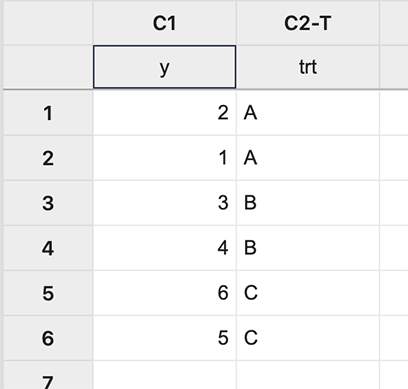
First input the data:
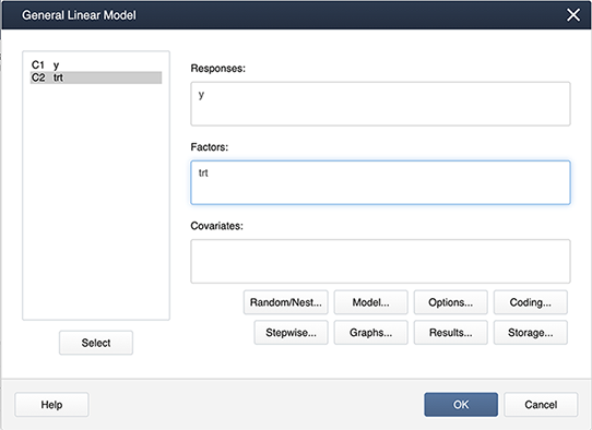
In Minitab, different coding options allow the choice of the design matrix which can be done as follows:
Stat > ANOVA > General Linear Model > Fit General Linear Model and place the variables in the appropriate boxes:
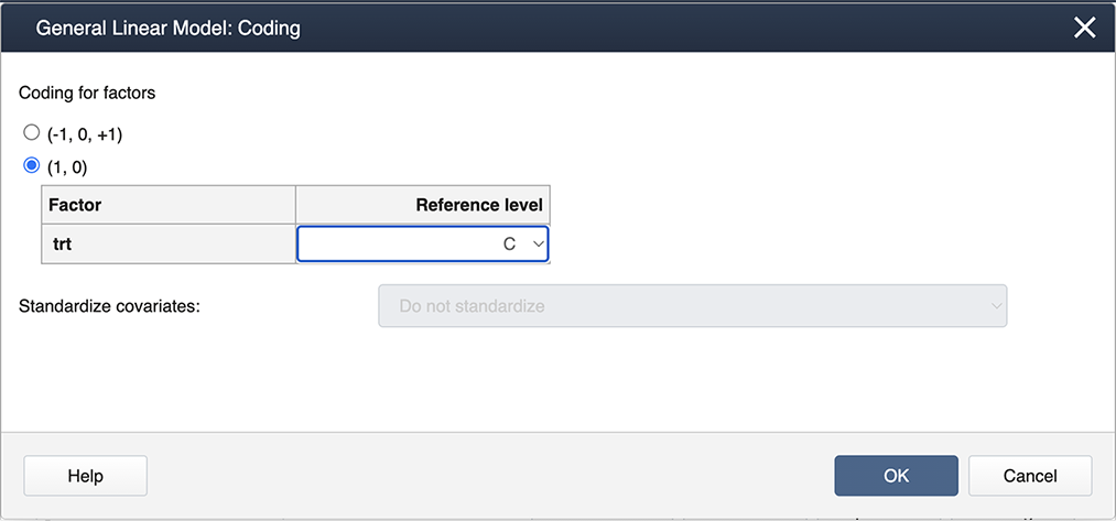
Then select Coding… and choose the (1,0) coding as shown below:
Analysis of Variance
| Source | DF | Adj SS | Adj MS | F-Value | P-Value |
|---|---|---|---|---|---|
| trt | 2 | 16.000 | 8.0000 | 16.00 | 0.025 |
| Error | 3 | 1.500 | 0.5000 | ||
| Total | 5 | 17.500 |
And also the Regression Equation:
Regression Equation
y = 5.500 - 4.000 trt_level1 - 2.000 trt_level2 + 0.0 trt_level3
First, we input the response variable and design matrix.
y = matrix(c(2,1,3,4,6,5), ncol=1)
x = matrix(c(1,1,0,1,1,0,1,0,1,1,0,1,1,0,0,1,0,0),6,3,byrow=TRUE)
x
      [,1] [,2] [,3]
[1,]    1    1    0
[2,]    1    1    0
[3,]    1    0    1
[4,]    1    0    1
[5,]    1    0    0
[6,]    1    0    0
Applying the same code as in Sections 4.2 and 4.3, we can then calculate the regression coefficients and create the ANOVA table.
beta = solve(t(x)%*%x)%*%(t(x)%*%y)
beta
     [,1]
[1,]  5.5
[2,] -4.0
[3,] -2.0
n = nrow(y)
p = ncol(x)
J = matrix(1,n,n)
ss_tot = (t(y)%*%y) - (1/n)*(t(y)%*%J)%*%y
ss_trt = t(beta)%*%(t(x)%*%y) - (1/n)*(t(y)%*%J)%*%y
ss_error = ss_tot - ss_trt
total_df = n-1
trt_df = p-1
error_df = n-p
MS_trt = ss_trt/(p-1)
MS_error = ss_error / error_df
Fstat = MS_trt/MS_error
ANOVA <- data.frame(
c ("","Treatment","Error", "Total"),
c("DF", trt_df,error_df,total_df),
c("SS", ss_trt, ss_error, ss_tot),
c("MS", MS_trt, MS_error, ""),
c("F",Fstat,"",""),
stringsAsFactors = FALSE)
names(ANOVA) <- c(" ", "  ", " ","","")
print(ANOVA, digits = 3)
1           DF   SS  MS  F
2 Treatment  2   16   8 16
3     Error  3  1.5 0.5
4     Total  5 17.5
The intermediate matrix computations can again be calculated with the following commands (outputs not shown).
xprimex = t(x)%*%x
xprimex
xprimey = t(x)%*%y
xprimey
xprimexinv = solve(t(x)%*%x)
xprimexinv
check = xprimexinv*xprimex
check
SumY2 = t(beta)%*%(t(x)%*%y)
SumY2
CF = (1/n)*(t(y)%*%J)%*%y
CF
R also uses indicator coding by default (option contr.treatment), however the default reference level is the first level (instead of the last as in SAS). For example, if we create a categorical variable with the levels and run the linear model, it is obvious from the coefficients that the first level is being used as the reference.
levels = c(1,1,2,2,3,3)
levels = as.factor(levels)
options(contrasts=c("contr.treatment","contr.poly"))
lm1 = lm(y~levels)
beta = lm1$coefficients
beta
(Intercept)     levels2     levels3
        1.5         2.0         4.0
To set the last (third) level as the reference, the command relevel must be used.
levels = relevel(levels,ref = "3")
lm2 = lm(y~levels)
beta = lm2$coefficients
beta
(Intercept)     levels1     levels2
        5.5        -4.0        -2.0
To obtain the ANOVA table, use the following commands.
library(car)
aov3 = Anova(lm2,type = 3) # identical to Anova(lm1,type = 3)
aov3
Anova Table (Type III tests)
Response: y
            Sum Sq Df F value   Pr(>F)
(Intercept)   60.5  1     121 0.001609 **
levels        16.0  2      16 0.025095 *
Residuals      1.5  3
---
Signif. codes:  0 ‘***’ 0.001 ‘**’ 0.01 ‘*’ 0.05 ‘.’ 0.1 ‘ ’ 1
In this case, the Type 3 ANOVA table is equivalent to the Type 1 table (output not shown).
aov1 = aov(lm2)
summary(aov1)