4: ANOVA Models Part II
4: ANOVA Models Part IIOverview
This is a continuation of the previous lesson, and in this lesson, three more alternative ANOVA models are introduced. ANOVA models are derived under the assumption of linearity of model parameters and additivity of model terms so that every model will follow the general linear model (GLM): \(Y=X\beta+\mathcal{E}\). In later sections of this lesson, we will see that the appropriate choice of \(X\), the design matrix, will result in a different ANOVA model. This lesson will also shed insight into the similarities of how ANOVA calculations are done by most software, regardless of which model is being used. Finally, the concept of a study diagram is discussed demonstrating its usefulness when building a statistical model and designing an experiment.
Objectives
- Apply the overall mean, cell means, and dummy variable regression models for a one-way ANOVA and interpret the results.
- Identify the design matrix and the parameter vector for each ANOVA model studied.
- Recognize aspects of ANOVA programming computations.
4.1 - The ANOVA Models
4.1 - The ANOVA ModelsIn this lesson, we will examine three new ANOVA models (Models 1, 2, 3), as well as the effects model (Model 4) from the previous lesson, defined as follows:
- Model 1 - The Overall Mean Model
- \(Y_{ij}=\mu+\epsilon_{ij}\)
-
which simply fits an overall or "grand mean". This model reflects the situation where \(H_0\) being true implies \(\mu_1=\mu_2=\cdots=\mu_T\).
- Model 2 - The Cell Means Model
- \(Y_{ij}=\mu_i+\epsilon_{ij}\)
-
where \(\mu_i\), \(i = 1,2, ...,T\) are the factor level means. Note that in this model, there is no overall mean being fitted.
- Model 3 - Dummy Variable Regression
- \(Y_{ij}=\mu+\mu_i+\epsilon_{ij}\), fitted as \(Y_{ij}=\beta_0+\beta_{Level1}+\beta_{Level2} \cdots \beta_{LevelT-1}+\epsilon_{ij}\)
-
where \(\beta_{Level1},\beta_{Level2}, ...,\beta_{LevelT-1}\) are regression coefficients for T-1 indicator-coded regression ‘dummy’ variables that correspond to the T-1 categorical factor levels. The Tth factor level mean is given by the regression intercept \(\beta_0\).
- Model 4 - The Effects Model
- \(Y_{ij}=\mu+\tau_i+\epsilon_{ij}\)
-
where \(\tau_i\) are the the deviations of each factor level mean from the overall mean so that \(\sum_{i=1}^T\tau_i=0\).
Each of these four models can be written as a general linear model (GLM): \(\mathbf{Y}=\mathbf{X}\boldsymbol{\beta}+\boldsymbol{\mathcal{E}}\) simply by changing the design matrix \(\mathbf{X}\). Thus to perform the data analysis, in terms of the computer coding instructions, the appropriate numerical values for the \(\mathbf{X}\) matrix elements will need to be inputted.
A note on how ANOVA is calculated: In the past lessons, we carried out the ANOVA computations conceptually in terms of deviations from means. For the calculation of total variance, we used the deviations of the individual observations from the overall mean, while the treatment SS was calculated using the deviations of treatment level means from the overall mean, and the residual or error SS was calculated using the deviations of individual observations from treatment level means. In practice, however, to achieve higher computational efficiency, SS for ANOVA is computed utilizing the following mathematical identity:
\(SS=\Sigma(Y_i-\bar{Y})^2=\Sigma Y_{i}^{2}-\dfrac{(\Sigma Y_i)^2}{N}\)
This identity is commonly called the "working formula" or "machine formula". The second term on the right-hand side is often referred to as the correction factor (CF).
When computing the SS for the total variance of the responses, the formula above can be used as it is, but modifications need be made for the others. For example, to compute the treatment SS, the above equation has to be modified as:
\(SS_{treatment} = \sum_{i=1}^{T}\dfrac{\left( \sum_{j=1}^{n_i}Y_{ij} \right)^2}{n_i}-\dfrac{(\sum_{i=1}^{T} \sum_{j=1}^{n_i} Y_{ij})^2}{N}\)
These working formulas will be utilized throughout the remaining course material.
4.2 - The Overall Mean Model
4.2 - The Overall Mean Model-
Model 1 - The Overall Mean Model
- \(Y_{ij}=\mu+\epsilon_{ij}\)
-
which simply fits an overall or "grand mean". This model reflects the situation where \(H_0\) being true implies \(\mu_1=\mu_2=\cdots=\mu_T\).
To understand how various facades of the model relate to each other, let us look at a toy example with 3 treatments (or factor levels) and 2 replicates of each treatment.
We have 6 observations, which means that \(\mathbf{Y}\) is a column vector of dimension 6 and so is the error vector \(\boldsymbol{\mathcal{E}}\) where its elements are the random error values associated with the 6 observations. In the GLM model, \(\mathbf{Y}=\mathbf{X}\boldsymbol{\beta}+\boldsymbol{\mathcal{E}}\), the design matrix \(\mathbf{X}\) for the overall mean model turns out to be a 6-dimensional column vector of ones. The parameter vector, \(\boldsymbol{\beta}\) is a scalar equal to \(\mu\), the overall population mean.
That is,
\(\mathbf{Y}=\begin{bmatrix}
2\\
1\\
3\\
4\\
6\\
5
\end{bmatrix} \text{,}\;\;\;\;
\mathbf{X}=\begin{bmatrix}
1\\
1\\
1\\
1\\
1\\
1
\end{bmatrix} \text{,}\;\;\;\;
\boldsymbol{\beta}=[\mu] \text{,}\;\;\;\; \text{ and }
\boldsymbol{\epsilon}=\begin{bmatrix}
\epsilon_1\\
\epsilon_2\\
\epsilon_3\\
\epsilon_4\\
\epsilon_5\\
\epsilon_6
\end{bmatrix}\)
Using the method of least squares, the estimates of the parameters in \(\boldsymbol{\beta}\) are obtained as:
\(\hat{\boldsymbol \beta}= (\mathbf{X}^{'} \mathbf{X} ) ^{-1} \mathbf{X}^{' } \mathbf{Y}\)
Using the estimate \(\hat{\boldsymbol{\beta}}\), the \(i^{th}\) predicted response \(\mathbf{\hat{y}}_i\) can be computed as \(\mathbf{\hat{y}}_i\)=\(\mathbf{x}_i^{'} \hat{\boldsymbol{\beta}} \) where \(\mathbf{x}_i^{'}\) denotes the \(i^{th}\) row vector of the design matrix.
In this simplest of cases, we can see how the matrix algebra works. The term \(\mathbf{X}^{'} \mathbf{X}\) would be:
\(\begin{bmatrix}
1 & 1 & 1 & 1 &1 & 1
\end{bmatrix}\ast \begin{bmatrix}
1\\
1\\
1\\
1\\
1\\
1
\end{bmatrix}=1+1+1+1+1+1=6 = n\)
The term \(\mathbf{X}^{'} \mathbf{Y}\) would be:
\(\begin{bmatrix}
1 & 1 & 1 & 1 &1 & 1
\end{bmatrix}\ast \begin{bmatrix}
2\\
1\\
3\\
4\\
5\\
6
\end{bmatrix}=2+1+3+4+5+6=21 = \Sigma Y_i\)
So in this case, the estimate \(\hat{\boldsymbol{\beta}}\) as expected is simply the overall mean = \(\hat{\boldsymbol{\mu}} = \bar{y}_{\cdot\cdot} = 21/6 = 3.5\)
Note that the exponent of \(\mathbf{X}^{'} \mathbf{X}\) in the formula above indicates arithmetic division as \(\mathbf{X}^{'} \mathbf{X}\) is a scalar in this case. In the more general setting, the superscript of '-1 ' indicates the inverse operation in matrix algebra.
To perform these matrix operations in SAS IML, we will open a regular SAS editor window, and then copy and paste three components from the file (IML Design Matrices):
Example
-
Step 1
Procedure initiation, and specification of the dependent variable vector, \(\mathbf{Y}\).
For our example we have:
/* Initiate IML, define response variable */ proc iml; y={ 2, 1, 3, 4, 6, 5}; -
Step 2
We then enter a design matrix (\(\mathbf{X}\)). For the Overall Mean model and our example data, we have:
x={ 1, 1, 1, 1, 1, 1}; -
Step 3
We can now copy and paste a program for the matrix computations to generate results (regression coefficients and ANOVA output):
beta=inv(x`*x)*x`*y;
beta_label={"Beta_0","Beta_1","Beta_2","Beta_3"};
print beta [label="Regression Coefficients"
rowname=beta_label];
n=nrow(y);
p=ncol(x);
j=j(n,n,1);
ss_tot = (y`*y) - (1/n)*(y`*j)*y;
ss_trt = (beta`*(x`*y)) - (1/n)*(y`*j)*y;
ss_error = ss_tot - ss_trt;
total_df=n-1;
trt_df=p-1;
error_df=n-p;
ms_trt = ss_trt/(p-1);
ms_error = ss_error / error_df;
F=ms_trt/ms_error;
empty={.};
row_label= {"Treatment", "Error", "Total"};
col_label={"df" "SS" "MS" "F"};
trt_row= trt_df || ss_trt || ms_trt || F;
error_row= error_df || ss_error || ms_error || empty;
tot_row=total_df || ss_tot || empty || empty;
aov = trt_row // error_row // tot_row;
print aov [label="ANOVA"
rowname=row_label
colname=col_label];
Here is a quick video walk-through to show you the process for how you can do this in SAS. (Right-click and select 'Show All' if your browser does not display the entire screencast window.)
The program can then be run to produce the following output:
| Regression Coefficients | |
|---|---|
| Beta_0 | 3.5 |
| ANOVA | ||||
|---|---|---|---|---|
| Treatment | DF | SS | MS | F |
| 0 | 0 | |||
| Error | 5 | 17.5 | 3.5 | |
| Total | 5 | 17.5 | ||
We see the estimate of the regression coefficient for \(\beta_0\) equals 3.5, which indeed is the overall mean of the response variable, and is also the same value we obtained above for \(\mu\) using 'by-hand' calculations. In this simple case, where the treatment factor has not entered the model, the only item of interest from the ANOVA table would be the \(SS_{Error}\) for later use in the General Linear F-test.
If you would like to see the internal calculations further, you may optionally add the following few lines, to the end of the calculation code.
 /* (Optional) Intermediates in the matrix computations */
xprimex=x`*x; print xprimex;
xprimey=x`*y; print xprimey;
xprimexinv=inv(x`*x); print xprimexinv;
check=xprimexinv*xprimex; print check;
SumY2=beta`*(x`*y); print SumY2;
CF=(1/n)*(y`*j)*y; print CF;
This additional code produces the following output:
| xprimex |
|---|
| 6 |
| xprimey |
|---|
| 21 |
| xprimexinv |
|---|
| 0.1666667 |
| check |
|---|
| 1 |
| SumY2 |
|---|
| 73.5 |
| CF |
|---|
| 73.5 |
For this model, we effectively have one treatment level \(T=1\) with six replicates \(n_1=N=6\). Using this and the formula for \(SS_{trt}\) at the bottom of the previous section, we can verify the computations for \(SS_{trt} = (\sum_{j=1}^{N}Y_{ij})^2 / N-CF = 0\).
The ‘check’ calculation confirms that \((\mathbf{X}^{'} \mathbf{X})^{-1}\mathbf{X}^{'}\mathbf{X} = 1\), which in fact defines the matrix division operation. In this simple case, it amounts to simple division by n but in other models that we will work with the matrix division process is more complicated. In general, the inverse of a matrix \(\mathbf{A}\) denoted \(\mathbf{A}^{-1}\), is defined by the matrix identity \(\mathbf{A}^{-1}\mathbf{A}=I\), where \(I\), is the identity matrix (a diagonal matrix of ‘1’s). In this example, \(\mathbf{A}\) is replaced by \(\mathbf{X}^{'}\mathbf{X}\), which is a scalar and equals 6.
First, we input the response variable and design matrix.
y = matrix(c(2,1,3,4,6,5), ncol=1)
x = matrix(c(1,1,1,1,1,1), ncol=1)
We can then calculate the regression coefficients.
beta = solve(t(x)%*%x)%*%(t(x)%*%y)
     [,1]
[1,]  3.5
Next we calculate the entries of the ANOVA Table.
n = nrow(y)
p = ncol(x)
J = matrix(1,n,n)
ss_tot = (t(y)%*%y) - (1/n)*(t(y)%*%J)%*%y
ss_trt = t(beta)%*%(t(x)%*%y) - (1/n)*(t(y)%*%J)%*%y
ss_error = ss_tot - ss_trt
total_df = n-1
trt_df = p-1
error_df = n-p
MS_trt = ss_trt/(p-1)
MS_error = ss_error / error_df
Fstat = MS_trt/MS_error
Then we can build and print the ANOVA table.
ANOVA <- data.frame(
c ("","Treatment","Error", "Total"),
c("DF", trt_df,error_df,total_df),
c("SS", ss_trt, ss_error, ss_tot),
c("MS", MS_trt, MS_error, ""),
c("F",Fstat,"",""),
stringsAsFactors = FALSE)
names(ANOVA) <- c(" ", "  ", " ","","")
print(ANOVA)
1           DF   SS  MS   F
2 Treatment  0    0 NaN NaN
3     Error  5 17.5 3.5
4     Total  5 17.5
The intermediate matrix computations can be calculated with the following commands (outputs not shown).
xprimex = t(x)%*%x
xprimex
xprimey = t(x)%*%y
xprimey
xprimexinv = solve(t(x)%*%x)
xprimexinv
check = xprimexinv*xprimex
check
SumY2 = t(beta)%*%(t(x)%*%y)
SumY2
CF = (1/n)*(t(y)%*%J)%*%y
CF
This model can be run with built-in R functions as follows:
options(contrasts=c("contr.sum","contr.poly"))
lm1 = lm(y~1)
beta = lm1$coefficients
beta
(Intercept)
3.5
To obtain the ANOVA table, use the following commands.
library(car)
aov3 = Anova(lm1,type = 3)
aov3
Anova Table (Type III tests)
Response: y
Sum Sq Df F value   Pr(>F)
(Intercept)   73.5  1      21 0.005934 **
Residuals     17.5  5
---
Signif. codes:  0 ‘***’ 0.001 ‘**’ 0.01 ‘*’ 0.05 ‘.’ 0.1 ‘ ’ 1
In this case, the Type 3 ANOVA table is equivalent to the Type 1 table.
aov1 = aov(lm1)
summary(aov1)
Df Sum Sq Mean Sq F value Pr(>F)
Residuals    5   17.5     3.5
4.3 - Cell Means Model
4.3 - Cell Means Model-
Model 2 - The Cell Means Model
- \(Y_{ij}=\mu_i+\epsilon_{ij}\)
-
where \(\mu_i\), \(i = 1,2, ...,T\) are the factor level means. Note that in this model, there is no overall mean being fitted.
The cell means model does not fit an overall mean, but instead fits an individual mean for each of the treatment levels. Let us examine this model for the same toy dataset assuming that a pair of observations arise from \(T = 3\) treatment levels. Each column will represent a specific treatment level using indicator coding, a ‘1’ for the rows corresponding to the observations receiving the specified treatment level, and a ‘0’ for the other rows.
To write the cell means model as a GLM, let \(\mathbf{X} = \begin{bmatrix} 1 & 0 & 0\\ 1 & 0 & 0 \\ 0 & 1 & 0 \\ 0 & 1 & 0 \\ 0 & 0 & 1 \\ 0 & 0 & 1 \end{bmatrix} = \begin{bmatrix} \mathbf{x}_1^{'} \\ \mathbf{x}_2^{'} \\ \mathbf{x}_3^{'} \\ \mathbf{x}_4^{'} \\ \mathbf{x}_5^{'} \\ \mathbf{x}_6^{'} \end{bmatrix}\), where \(\mathbf{x}_i^{'}\) is the \(i^{th}\) row vector of the design matrix. It can be seen that \(r=2\) is the number of replicates for each treatment level. Observe that column 1 generates the mean for treatment level 1, column 2 for treatment level 2, and column 3 for treatment level 3.
The parameter vector \(\boldsymbol{\beta}\) is a 3-dimensional column vector and is defined by,
\(\boldsymbol{\beta}= \begin{bmatrix}
\beta_0\\
\beta_1\\
\beta_2
\end{bmatrix} = \begin{bmatrix}
\mu_1\\
\mu_2\\
\mu_3
\end{bmatrix}.\)
The parameter estimates \(\hat{\boldsymbol{\beta}}\) can again be found using the least squares method. One can verify that \(\mu_{i} = \bar{y}_i\), the \(i^{th}\) treatment mean, for \(i=1,2,3\). Using this estimate, the resulting estimated regression equation for the cell means model is,
\(\hat{\mathbf{Y}} = \mathbf{X}\hat{\boldsymbol{\beta}}\)
which produces \(\hat{\mathbf{y}}_i = \mathbf{x}_i^{'}\begin{bmatrix} \hat{\mu}_1 \\ \hat{\mu}_2 \\ \hat{\mu}_3 \end{bmatrix}\).
Using Technology
Begin by replacing the design matrix in the IML code of Section 4.2 Step 2 with:
/* The Cell Means Model */
x={
1	0	0,
1	0	0,
0	1	0,
0	1	0,
0	0	1,
0	0	1};
We then re-run the program with the new design matrix to get the following output:
| Regression Coefficients | |
|---|---|
| Beta_0 | 1.5 |
| Beta_1 | 3.5 |
| Beta_2 | 5.5 |
| ANOVA | ||||
|---|---|---|---|---|
| Treatment | dF | SS | MS | F |
| 2 | 16 | 8 | 16 | |
| Error | 3 | 1.5 | 0.5 | |
| Total | 5 | 17.5 | ||
The regression coefficients Beta_0, Beta_1, and Beta_2 are now the means for each treatment level, and in the ANOVA table, we see that the \(SS_{Error}\) (SSE) is 1.5. This reduction in the SSE is the \(SS_{trt}\). Notice that the error SS of the 'Overall Mean' model is the sum of the SS values for Treatment and Error term in this model, which means that by not including the treatment effect in that model, its error SS has been unduly inflated.
Adding the optional code given in Section 4.2 to compute additional internal computations, we can obtain:
| xprimex | ||
|---|---|---|
| 2 | 0 | 0 |
| 0 | 2 | 0 |
| 0 | 0 | 2 |
| check | ||
|---|---|---|
| 1 | 0 | 0 |
| 0 | 1 | 0 |
| 0 | 0 | 1 |
| xprimey |
|---|
| 3 |
| 7 |
| 11 |
| SumY2 |
|---|
| 89.5 |
| CF |
|---|
| 73.5 |
| xprimexinv | ||
|---|---|---|
| 0.5 | 0 | 0 |
| 0 | 0.5 | 0 |
| 0 | 0 | 0.5 |
Here we can see that \(\mathbf{X}^{'}\mathbf{X}\) now contains diagonal elements that are the \(n_i\) = number of observations for each treatment level mean being computed. In addition, we can use the ‘working formula’ to verify the treatment SS is \(89.5 - 73.5 = 16\).
We can now test for the significance of the treatment by using the General Linear F-test:
\(F=\dfrac{(SSE_{reduced} - SSE_{full})/(dfE_{reduced} - dfE_{full})}{SSE_{full} / dfE_{full}}\)
The 'Overall Mean' model is the 'Reduced' model, and the 'Cell Means' model is the ‘Full’ model. From the ANOVA tables, we get:
\(F=\dfrac{17.5-1.5⁄5-3}{1.5⁄3}=16\)
which can be compared to \(F_{0.05,2,3}=9.55\).
First, we input the response variable and design matrix.
y = matrix(c(2,1,3,4,6,5), ncol=1)
x = matrix(c(1,0,0,1,0,0,0,1,0,0,1,0,0,0,1,0,0,1),6,3,byrow=TRUE)
x
     [,1] [,2] [,3]
[1,]    1    0    0
[2,]    1    0    0
[3,]    0    1    0
[4,]    0    1    0
[5,]    0    0    1
[6,]    0    0    1
Applying the same code as in Section 4.2, we can then calculate the regression coefficients and create the ANOVA table.
beta = solve(t(x)%*%x)%*%(t(x)%*%y)
beta
     [,1]
[1,]  1.5
[2,]  3.5
[3,]  5.5
n = nrow(y)
p = ncol(x)
J = matrix(1,n,n)
ss_tot = (t(y)%*%y) - (1/n)*(t(y)%*%J)%*%y
ss_trt = t(beta)%*%(t(x)%*%y) - (1/n)*(t(y)%*%J)%*%y
ss_error = ss_tot - ss_trt
total_df = n-1
trt_df = p-1
error_df = n-p
MS_trt = ss_trt/(p-1)
MS_error = ss_error / error_df
Fstat = MS_trt/MS_error

ANOVA <- data.frame(
  c ("","Treatment","Error", "Total"),
  c("DF", trt_df,error_df,total_df),
  c("SS", ss_trt, ss_error, ss_tot),
  c("MS", MS_trt, MS_error, ""),
  c("F",Fstat,"",""),
  stringsAsFactors = FALSE)
names(ANOVA) <- c(" ", "  ", " ","","")
print(ANOVA)
1           DF   SS  MS  F
2 Treatment  2   16   8 16
3     Error  3  1.5 0.5
4     Total  5 17.5
The intermediate matrix computations can again be calculated with the following commands (outputs not shown).
xprimex = t(x)%*%x
xprimex
xprimey = t(x)%*%y
xprimey
xprimexinv = solve(t(x)%*%x)
xprimexinv
check = xprimexinv*xprimex
check
SumY2 = t(beta)%*%(t(x)%*%y)
SumY2
CF = (1/n)*(t(y)%*%J)%*%y
CF
Creating a categorical variable with the levels, this model can be run with built in R functions as follows:
levels = c(1,1,2,2,3,3)
levels = as.factor(levels)
lm1 = lm(y~ -1 + levels)
beta = lm1$coefficients
beta
levels1 levels2 levels3
    1.5     3.5     5.5
To obtain the ANOVA table, use the following commands.
options(contrasts=c("contr.sum","contr.poly"))
library(car)
aov3 = Anova(lm(y~levels),type = 3)
aov3
Anova Table (Type III tests)

Response: y
            Sum Sq Df F value   Pr(>F)
(Intercept)   73.5  1     147 0.001208 **
levels        16.0  2      16 0.025095 *
Residuals      1.5  3
---
Signif. codes:  0 ‘***’ 0.001 ‘**’ 0.01 ‘*’ 0.05 ‘.’ 0.1 ‘ ’ 1
Again, the Type 3 ANOVA table is equivalent to the Type 1 table for this model.
aov1 = aov(lm(y~levels))
summary(aov1)
          Df Sum Sq Mean Sq F value Pr(>F)
levels     2   16.5     8.0      16 0.0251 *
Residuals  3    1.5     0.5
---
Signif. codes:  0 ‘***’ 0.001 ‘**’ 0.01 ‘*’ 0.05 ‘.’ 0.1 ‘ ’ 1
4.4 - Dummy Variable Regression
4.4 - Dummy Variable Regression-
Model 3 - Dummy Variable Regression
- \(Y_{ij}=\mu+\mu_i+\epsilon_{ij}\), fitted as \(Y_{ij}=\beta_0+\beta_{Level1}+\beta_{Level2}+ \cdots +\beta_{LevelT-1}+\epsilon_{ij}\)
-
where \(\beta_{Level1},\beta_{Level2}, ...,\beta_{LevelT-1}\) are regression coefficients for T-1 indicator-coded regression ‘dummy’ variables that correspond to the T-1 categorical factor levels. The Tth factor level mean is given by the regression intercept \(\beta_0\).
The GLM applied to data with categorical predictors can be viewed from a regression modeling perspective as an ordinary multiple linear regression (MLR) with ‘dummy’ coding, also known as indicator coding, for the categorical treatment levels. Typically software performing the MLR will automatically include an intercept, which corresponds to the first column of the design matrix and is a column of 1's. This automatic inclusion of the intercept can lead to complications when interpreting the regression coefficients (discussed below).
Consider again the toy example with a pair of observations from 3 different treatment levels. The design matrix for this dummy variable model is as follows:
\(\bf{X} = \begin{bmatrix}
1 & 1 & 0 \\
1 & 1 & 0 \\
1 & 0 & 1 \\
1 & 0 & 1 \\
1 & 0 & 0 \\
1 & 0 & 0
\end{bmatrix} \)
Notice that in the above design matrix, there are only two indicator columns even though there are three treatment levels in the study. If we were to have a design matrix with another indicator column representing the third treatment level (as seen below), the resulting 4 columns would form a set of linearly dependent columns, a mathematical condition which hinders the computation process any further. This over-parameterized design matrix would look as follows:
\(\bf{X} = \begin{bmatrix}
1 & 1 & 0 & 0 \\
1 & 1 & 0 & 0\\
1 & 0 & 1 & 0\\
1 & 0 & 1 & 0\\
1 & 0 & 0 & 1\\
1 & 0 & 0 & 1
\end{bmatrix} \)
This matrix containing all 4 columns has the property that the sum of columns 2, 3, and 4 will equal the first column representing the intercept. As a result, the matrix is what is known as 'singular' and the matrix computations will not run. To remedy this, one of the treatment levels is omitted from the coding in the correct design matrix above and the eliminated level is called the ‘reference’ level. In SAS, typically, the treatment level with the highest label is defined as the reference level (treatment level 3 in our example).
Note that the parameter vector for the dummy variable regression model is, \(\boldsymbol{\beta} = \begin{bmatrix}
\mu\\
\mu_1\\
\mu_2
\end{bmatrix}\)
Using Technology
The SAS Mixed procedure (and the GLM procedure which we may encounter later) use the 'Dummy Variable Regression' model by default. For the data used in sections 4.2 and 4.3, the design matrix for this model can be entered into IML as:
/* Dummy Variable Regression Model */
x = {
1	1	0,
1	1	0,
1	0	1,
1	0	1,
1   	0   	0,
1   	0   	0};
Running IML, with the design matrix for the dummy variable regression model, we get the following output;
| Regression Coefficients | |
|---|---|
| Beta_0 | 5.5 |
| Beta_1 | -4 |
| Beta_2 | -2 |
The coefficient \(\beta_0\) is the mean for treatment level3. The mean for treatment level1 is then calculated from \(\hat{\beta}_0+\hat{\beta}_1=1.5\). Likewise, the mean for treatment level2 is calculated as \(\hat{\beta}_0+\hat{\beta}_2=3.5\).
Notice that the F statistic calculated from this model is the same as that produced from the Cell Means model.
| ANOVA | ||||
|---|---|---|---|---|
| Treatment | df | SS | MS | F |
| 2 | 16 | 8 | 16 | |
| Error | 3 | 1.5 | 0.5 | |
| Total | 5 | 17.5 | ||
In SAS, the default coding is indicator coding, so when you specify the option
model y=trt / solution;
you get the regression coefficients:
| Solution for Fixed Effects | ||||||
|---|---|---|---|---|---|---|
| Effect | trt | Estimate | Standard Error | DF | t Value | Pr > |t| |
| Intercept | 5.5000 | 0.5000 | 3 | 11.00 | 0.0016 | |
| trt | level1 | -4.0000 | 0.7071 | 3 | -5.66 | 0.0109 |
| trt | level2 | -2.0000 | 0.7071 | 3 | -2.83 | 0.0663 |
| trt | level3 | 0 | ||||
And the same ANOVA table:
| Type 3 Analysis of Variance | ||||||||
|---|---|---|---|---|---|---|---|---|
| Source | DF | Sum of Squares | Mean Square | Expected Mean Square | Error Term | Error DF | F Value | Pr > F |
| trt | 2 | 16.000000 | 8.000000 | Var(Residual)+Q(trt) | MS(Residual) | 3 | 16.00 | 0.0251 |
| Residual | 3 | 1.500000 | 0.500000 | Var(Residual) | ||||
The Intermediate calculations for this model are:
| xprimex | ||
|---|---|---|
| 6 | 2 | 2 |
| 2 | 2 | 0 |
| 2 | 0 | 2 |
| check | ||
|---|---|---|
| 1 | -2.22E-16 | 0 |
| 3.331E-16 | 1 | 0 |
| 0 | 0 | 1 |
| xprimey |
|---|
| 21 |
| 3 |
| 7 |
| SumY2 |
|---|
| 89.5 |
| CF |
|---|
| 73.5 |
| xprimexinv | ||
|---|---|---|
| 0.5 | -0.5 | -0.5 |
| -0.5 | 1 | 0.5 |
| -0.5 | 0.5 | 1 |
We can confirm our ANOVA table now by running the analysis in software such as Minitab.
First input the data:
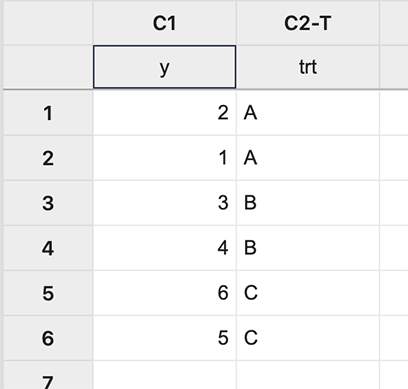
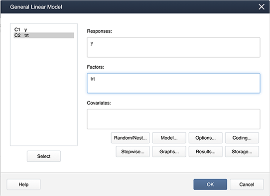
In Minitab, different coding options allow the choice of the design matrix which can be done as follows:
Stat > ANOVA > General Linear Model > Fit General Linear Model and place the variables in the appropriate boxes:
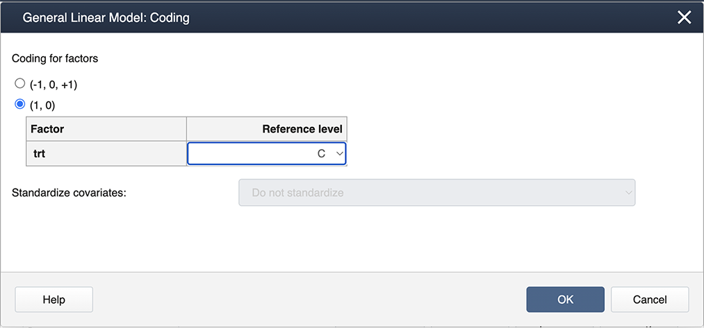
Then select Coding… and choose the (1,0) coding as shown below:
Analysis of Variance
| Source | DF | Adj SS | Adj MS | F-Value | P-Value |
|---|---|---|---|---|---|
| trt | 2 | 16.000 | 8.0000 | 16.00 | 0.025 |
| Error | 3 | 1.500 | 0.5000 | ||
| Total | 5 | 17.500 |
And also the Regression Equation:
Regression Equation
y = 5.500 - 4.000 trt_level1 - 2.000 trt_level2 + 0.0 trt_level3
First, we input the response variable and design matrix.
y = matrix(c(2,1,3,4,6,5), ncol=1)
x = matrix(c(1,1,0,1,1,0,1,0,1,1,0,1,1,0,0,1,0,0),6,3,byrow=TRUE)
x
      [,1] [,2] [,3]
[1,]    1    1    0
[2,]    1    1    0
[3,]    1    0    1
[4,]    1    0    1
[5,]    1    0    0
[6,]    1    0    0
Applying the same code as in Sections 4.2 and 4.3, we can then calculate the regression coefficients and create the ANOVA table.
beta = solve(t(x)%*%x)%*%(t(x)%*%y)
beta
     [,1]
[1,]  5.5
[2,] -4.0
[3,] -2.0
n = nrow(y)
p = ncol(x)
J = matrix(1,n,n)
ss_tot = (t(y)%*%y) - (1/n)*(t(y)%*%J)%*%y
ss_trt = t(beta)%*%(t(x)%*%y) - (1/n)*(t(y)%*%J)%*%y
ss_error = ss_tot - ss_trt
total_df = n-1
trt_df = p-1
error_df = n-p
MS_trt = ss_trt/(p-1)
MS_error = ss_error / error_df
Fstat = MS_trt/MS_error
ANOVA <- data.frame(
c ("","Treatment","Error", "Total"),
c("DF", trt_df,error_df,total_df),
c("SS", ss_trt, ss_error, ss_tot),
c("MS", MS_trt, MS_error, ""),
c("F",Fstat,"",""),
stringsAsFactors = FALSE)
names(ANOVA) <- c(" ", "  ", " ","","")
print(ANOVA, digits = 3)
1           DF   SS  MS  F
2 Treatment  2   16   8 16
3     Error  3  1.5 0.5
4     Total  5 17.5
The intermediate matrix computations can again be calculated with the following commands (outputs not shown).
xprimex = t(x)%*%x
xprimex
xprimey = t(x)%*%y
xprimey
xprimexinv = solve(t(x)%*%x)
xprimexinv
check = xprimexinv*xprimex
check
SumY2 = t(beta)%*%(t(x)%*%y)
SumY2
CF = (1/n)*(t(y)%*%J)%*%y
CF
R also uses indicator coding by default (option contr.treatment), however the default reference level is the first level (instead of the last as in SAS). For example, if we create a categorical variable with the levels and run the linear model, it is obvious from the coefficients that the first level is being used as the reference.
levels = c(1,1,2,2,3,3)
levels = as.factor(levels)
options(contrasts=c("contr.treatment","contr.poly"))
lm1 = lm(y~levels)
beta = lm1$coefficients
beta
(Intercept)     levels2     levels3
        1.5         2.0         4.0
To set the last (third) level as the reference, the command relevel must be used.
levels = relevel(levels,ref = "3")
lm2 = lm(y~levels)
beta = lm2$coefficients
beta
(Intercept)     levels1     levels2
        5.5        -4.0        -2.0
To obtain the ANOVA table, use the following commands.
library(car)
aov3 = Anova(lm2,type = 3) # identical to Anova(lm1,type = 3)
aov3
Anova Table (Type III tests)
Response: y
            Sum Sq Df F value   Pr(>F)
(Intercept)   60.5  1     121 0.001609 **
levels        16.0  2      16 0.025095 *
Residuals      1.5  3
---
Signif. codes:  0 ‘***’ 0.001 ‘**’ 0.01 ‘*’ 0.05 ‘.’ 0.1 ‘ ’ 1
In this case, the Type 3 ANOVA table is equivalent to the Type 1 table (output not shown).
aov1 = aov(lm2)
summary(aov1)
4.5 - The Effects Model
4.5 - The Effects Model-
Model 4 - The Effects Model
- \(Y_{ij}=\mu+\tau_i+\epsilon_{ij}\)
-
where \(\tau_i\) are the deviations of each factor level mean from the overall mean so that \(\sum_{i=1}^T\tau_i=0\).
In the effects model that we discussed in lesson 3, the treatment means were not estimated, but instead, the deviations of treatment means from the overall mean were estimated (the \(\tau_i\)'s). The model must include the overall mean, thus we need to include \(\mu_., \tau_1 , ... , \tau_T\) as elements in the parameter vector, \(\boldsymbol{\beta}\) of the GLM model. Note that, in the case of equal replication at each factor level, the deviations satisfy the following constraint:
\(\sum_{i=1}^{T} \tau_i =0\)
This implies that one of the \(\tau_i\) parameters is not needed since it can be expressed in terms of the other T - 1 parameters and need not be included in the \(\boldsymbol{\beta}\) parameter vector. We shall drop the parameter \(\tau_T\) from the regression equation as it can be expressed in terms of the other T - 1 parameters \(\tau_i\) as follows:
\(\tau_T\ = -\tau_1 - \tau_2 - \cdots \tau_{T-1}\)
Thus, the \(\boldsymbol{\beta}\) vector of the GLM is a \(T \times 1\) vector containing only the parameters \(\mu, \tau_1 , ... , \tau_{T-1}\) for the linear model.
To illustrate how a linear model is developed with this approach, consider again a single-factor study with T = 3 factor levels with \(n_1=n_2=n_3=2\). The \(\mathbf{Y}\), \(\mathbf{X}\), \(\boldsymbol{\beta}\) and \(\boldsymbol{\epsilon}\) matrices for this case are as follows:
\(\mathbf{Y} = \begin{bmatrix}Y_{11}\\ Y_{12}\\ Y_{21}\\ Y_{22}\\ Y_{31}\\ Y_{32}\end{bmatrix}\text{, }\mathbf{X} = \begin{bmatrix}1 & 1 & 0\\ 1 & 1 & 0\\ 1 & 0 & 1\\ 1 & 0 & 1\\ 1 & -1 & -1\\ 1 & -1 & -1\end{bmatrix}\text{, }\boldsymbol{\beta} = \begin{bmatrix}\beta_{0}\\ \beta_{1}\\ \beta_{2}\end{bmatrix}\text{, and } \boldsymbol{\epsilon} = \begin{bmatrix}\epsilon_{11}\\ \epsilon_{12}\\ \epsilon_{21}\\ \epsilon_{22}\\ \epsilon_{31}\\ \epsilon_{32}\end{bmatrix}\)
where \(\beta_0, \beta_1 \text{ and } \beta_2\), corresponds to \(\mu, \tau_1 \text{ and } \tau_2\) respectively.
Note that the vector of expected values \(\mathbf{E}\{\mathbf{Y}\} =\mathbf{X}\boldsymbol{\beta}\), yields the following:
\begin{aligned} \mathbf{E}\{\mathbf{Y}\} &= \mathbf{X}\boldsymbol{\beta} \\ \begin{bmatrix}E\{Y_{11}\}\\ E\{Y_{12}\}\\ E\{Y_{21}\}\\ E\{Y_{22}\}\\E\{Y_{31}\}\\E\{Y_{32}\}\end{bmatrix} &= \begin{bmatrix}1 & 1 & 0\\ 1 & 1 & 0\\ 1 & 0 & 1\\ 1 & 0 & 1\\ 1 & -1 & -1\\ 1 & -1 & -1\end{bmatrix}\begin{bmatrix}\beta_{0}\\ \beta_{1}\\ \beta_{2}\end{bmatrix} \\ &= \begin{bmatrix}\mu_{.}+\tau_{1}\\ \mu+\tau_{1}\\ \mu+\tau_{2}\\ \mu+\tau_{2}\\ \mu-\tau_{1}-\tau_{2}\\ \mu-\tau_{1}-\tau_{2}\end{bmatrix} \end{aligned}
Since \(\tau_3=-\tau_{1}-\tau_{2}\), see above, we see that \(E\{Y_{31}\} =E\{Y_{32}\}=\mu+\tau_{3}\). Thus, the above \(\mathbf{X}\) matrix and \(\boldsymbol{\beta}\) vector representation provides the appropriate expected values for all factor levels as expressed below:
\(E\{Y_{ij}\} =\mu+\tau_{i}\)
Using Technology
Begin by replacing the design matrix in the IML code of Section 4.2 Step 2 with:
/* The Effects Model */
x={
1	1	0,
1	1	0,
1	0	1,
1	0	1,
1	-1	-1,
1	-1	-1};
Here we have another omission of a treatment level, but for a different reason. In the effects model, we have the constraint \(\Sigma \tau_i =0\). As a result, coding for one treatment level can be omitted.
Running the IML program with this design matrix yields:
| Regression Coefficients | |
|---|---|
| Beta_0 | 3.5 |
| Beta_1 | -2 |
| Beta_2 | 0 |
| ANOVA | ||||
|---|---|---|---|---|
| Treatment | dF | SS | MS | F |
| 2 | 16 | 8 | 16 | |
| Error | 3 | 1.5 | 0.5 | |
| Total | 5 | 17.5 | ||
The regression coefficient Beta_0 is the overall mean and the coefficients \(\beta_1\) and \(\beta_2\) are \(\tau_1\) and \(\tau_2\) respectively. The estimate for \(\tau_3\) is obtained as \(– (\tau_1)-( \tau_2) = 2.0\).
In Minitab, if we change the coding now to be Effect coding (-1,0,+1), which is the default setting, we get the following:
Regression Equation
y = 3.500 - 2.000 trt_A - 0.000 trt_B + 2.000 trt_C
The ANOVA table is the same as for the dummy-variable regression model above. We can also observe that the factor level means and General Linear F Statistics values obtained for all 3 representations (cell means, dummy coded regression and effects coded regression) are identical, confirming that the 3 representations are identical.
The intermediates were:
| xprimex | ||
|---|---|---|
| 6 | 0 | 0 |
| 0 | 4 | 2 |
| 0 | 2 | 4 |
| check | ||
|---|---|---|
| 1 | 0 | 0 |
| 0 | 1 | 0 |
| 0 | 0 | 1 |
| xprimey |
|---|
| 21 |
| -8 |
| -4 |
| SumY2 |
|---|
| 89.5 |
| CF |
|---|
| 73.5 |
| xprimexinv | ||
|---|---|---|
| 0.1666667 | 0 | 0 |
| 0 | 0.3333333 | -0.166667 |
| 0 | -0.166667 | 0.3333333 |
First, we input the response variable and design matrix.
y = matrix(c(2,1,3,4,6,5), ncol=1)
x = matrix(c(1,1,0,1,1,0,1,0,1,1,0,1,1,-1,-1,1,-1,-1),6,3,byrow=TRUE)
x
     [,1] [,2] [,3]
[1,]    1    1    0
[2,]    1    1    0
[3,]    1    0    1
[4,]    1    0    1
[5,]    1   -1   -1
[6,]    1   -1   -1
Applying the same code as in the previous sections, we can then calculate the regression coefficients and create the ANOVA table.
beta = solve(t(x)%*%x)%*%(t(x)%*%y)
beta
     [,1]
[1,]  3.5
[2,] -2.0
[3,]  0.0
n = nrow(y)
p = ncol(x)
J = matrix(1,n,n)
ss_tot = (t(y)%*%y) - (1/n)*(t(y)%*%J)%*%y
ss_trt = t(beta)%*%(t(x)%*%y) - (1/n)*(t(y)%*%J)%*%y
ss_error = ss_tot - ss_trt
total_df = n-1
trt_df = p-1
error_df = n-p
MS_trt = ss_trt/(p-1)
MS_error = ss_error / error_df
Fstat = MS_trt/MS_error

ANOVA <- data.frame(
  c ("","Treatment","Error", "Total"),
  c("DF", trt_df,error_df,total_df),
  c("SS", ss_trt, ss_error, ss_tot),
  c("MS", MS_trt, MS_error, ""),
  c("F",Fstat,"",""),
  stringsAsFactors = FALSE)
names(ANOVA) <- c(" ", "  ", " ","","")
print(ANOVA, digits = 3)
1           DF   SS  MS  F
2 Treatment  2   16   8 16
3     Error  3  1.5 0.5
4     Total  5 17.5
The intermediate matrix computations can again be calculated with the following commands (outputs not shown).
xprimex = t(x)%*%x
xprimex
xprimey = t(x)%*%y
xprimey
xprimexinv = solve(t(x)%*%x)
xprimexinv
check = xprimexinv*xprimex
check
SumY2 = t(beta)%*%(t(x)%*%y)
SumY2
CF = (1/n)*(t(y)%*%J)%*%y
CF
To use effect coding in R, we can specify the “sum contrast” option within the lm function as follows.
levels = c(1,1,2,2,3,3)
levels = as.factor(levels)
lm1 = lm(y~levels,contrasts = list(levels = contr.sum))
beta = lm1$coefficients
round(beta,1) # rounding to one decimal point
(Intercept)     levels1     levels2
        3.5        -2.0         0.0
We can then obtain the Type 3 ANOVA table (again, equivalent to the Type 1 in this case; outputs not shown).
aov3 = car::Anova(lm1,type = 3) # syntax alternative to loading the car package
aov3
4.6 - The Study Diagram
4.6 - The Study DiagramIn Lesson 1.1 we encountered a brief description of an experiment. The description of an experiment provides a context for understanding how to build an appropriate statistical model. All too often mistakes are made in statistical analyses because of a lack of understanding of the setting and procedures in which a designed experiment is conducted. Creating a study diagram is one of the best and intuitive ways to address this. A study diagram is a schematic diagram that captures the essential features of the experimental design. Here, as we explore the computations for a single factor ANOVA in a simple experimental setting, the study diagram may seem trivial. However, in practice and in lessons to follow, the ability to create an accurate study diagram usually makes a substantial difference in getting the model right.
In our example in Lesson 1.1, a plant biologist thinks that plant height may be affected by the fertilizer type and three types of fertilizer were chosen to investigate this claim. Next, 24 plants were randomly chosen and 4 batches of 6 plants each were assigned to the 3 fertilizer types and as well as a control (untreated) group. The individual plants were randomly assigned the treatment levels to produce 6 replications within each level. The researchers kept all the plants under equivalent conditions in a single greenhouse throughout the experiment. Here is the resulting data:
Control | F1 | F2 | F3 |
|---|---|---|---|
21 | 32 | 22.5 | 28 |
19.5 | 30.5 | 26 | 27.5 |
22.5 | 25 | 28 | 31 |
21.5 | 27.5 | 27 | 29.5 |
20.5 | 28 | 26.5 | 30 |
21 | 28.6 | 25.2 | 29.2 |
We have a description of the treatment levels, how they were assigned to individual experimental units (the potted plant), and we can see the data organized in a table... What are we missing? A key question is: how was the experiment conducted? This question is a practical one and is answered with a study diagram. These are usually hand-drawn depictions of a real setting, indicating the treatments, levels of treatments, and how the experiment was laid out. For this example, we need to draw a greenhouse bench, capable of holding the 4 × 6 = 24 experimental units:
The diagram identified the response variable, listed the treatment levels, and indicated the random assignment of treatment levels to these 24 experimental units on the greenhouse bench.
This randomization and the subsequent experimental layout we would identify as a Completely Randomized Design (CRD). We know from this schematic diagram that we need a statistical model that is appropriate for a one-way ANOVA in a Completely Randomized Design (CRD).
Furthermore, once the plant heights are recorded at the end of the study, the experimenter may observe that the variability in the growth may be influenced by additional factors besides the fertilizer level (e.g. position on the bench). A careful examination of the layout of the plants in the study diagram may perhaps reveal this additional factor. For example, if the growth is higher in the plants placed on the row nearer to the windows, it is reasonable to assume that sunlight also plays a role. In this case, an experimenter may redesign the experiment as a randomized completely block design (RCBD) with rows as a blocking factor. Note that design aspects of experiments (such as CRD and RCBD) are covered in Lessons 7 and 8.
Being able to draw and reproduce a study diagram is very useful in identifying the components of the ANOVA models.
4.7 - Try it!
4.7 - Try it!Exercise 1: Design Matrix
Below is a design matrix for a data set of a recent study.
\[ \begin{pmatrix} 1 & 1 & 0 & 0\\ 1 & 1 & 0 & 0\\ 1 & 1 & 0 & 0\\ 1 & 0 & 1 & 0 \\1 & 0 & 1 & 0\\1 & 0 & 1 & 0\\1 & 0 & 0 & 1\\1 & 0 & 0 & 1\\1 & 0 & 0 & 1\\1 & -1 & -1 & -1\\1 & -1 & -1 & -1\\1 & -1 & -1 & -1\end{pmatrix} \]
- Identify the number of treatment levels and replicates.
4 treatment levels and 3 replicates
- Name the model and write its equation.
This design matrix corresponds to the effects model and the model equation is \(Y_{ij}=\mu+\tau_i+\epsilon_{ij}\), where i = 1 to 4; j = 1 to 3 and \(\sum_{i=1}^4 \tau_i = 0\).
- Write the equation and the design matrix that corresponds to the cell means model.
The equation for the cell means model is: \(Y_{ij}=\mu_{i}+\epsilon_{ij}\) where i = 1 to 4 and j = 1 to 3. The design matrix corresponding to the cell means model is:
\[ \begin{pmatrix} 1 & 0 & 0 & 0\\ 1 & 0 & 0 & 0\\ 1 & 0 & 0 & 0\\ 0 & 1 & 0 & 0 \\0 & 1 & 0 & 0\\0 & 1 & 0 & 0\\0 & 0 & 1 & 0\\0 & 0 & 1 & 0\\0 & 0 & 1 & 0\\0 & 0 & 0 & 1\\0 & 0 & 0 & 1\\0 & 0 & 0 & 1\end{pmatrix} \]
- Write the equation and the design matrix that corresponds to the dummy variable regressions model.
The equation for the 'dummy variable regression' model is: \(Y_{ij} = \mu + \mu_i+\epsilon_{ij}\) for i = 1 to 3 and j = 1 to 3.
\(Y_{4j}=\mu + \epsilon_{4j}\)
The design matrix is given below. Note that the last 3 rows correspond to the 4th treatment level which is the reference category and its effect is estimated by the model intercept.
\[ \begin{pmatrix} 1 & 1 & 0 & 0\\ 1 & 1 & 0 & 0\\ 1 & 1 & 0 & 0\\ 1 & 0 & 1 & 0 \\1 & 0 & 1 & 0\\1 & 0 & 1 & 0\\1 & 0 & 0 & 1\\1 & 0 & 0 & 1\\1 & 0 & 0 & 1\\1 & 0 & 0 & 0\\1 & 0 & 0 & 0\\1 & 0 & 0 & 0\end{pmatrix} \]
4.8 - Lesson 4 Summary
4.8 - Lesson 4 SummaryThis lesson covered four different versions of single-factor ANOVA models. They are: Overall Mean, Cell Means, Dummy Variable Regression, and Effects Coded Regression models. This lesson also provided the coding compatible with the SAS IML procedure, which facilitates the ANOVA computations using Matrix Algebra in a GLM setting. The method of least squares was used to estimate model parameters yielding a prediction equation for the response in terms of the treatment level. This prediction tool will show to be more useful in ANCOVA settings where model predictors are both categorical and numerical (more details on ANCOVA in Lessons 9 and 10). The prediction process can be utilized effectively only with a sound knowledge of the parameterization process for each ANOVA model. To facilitate this understanding, the models were run with IML code and the resulting parameter vector was used for interpreting the prediction (regression) equations.
Finally, using the greenhouse example, the concept of a study diagram was discussed. Though a simple visual tool, a study diagram may play an important role in identifying new predictors so that a pre-determined ANOVA model can be extended to include additional factors creating a multi-factor model (discussed in Lessons 5 and 6). In addition to identifying the treatment design, the study diagram also helps in choosing an appropriate randomization design (a topic discussed in Lessons 7 and 8).