3.2 - Sample Size Determination
3.2 - Sample Size DeterminationAn important aspect of designing an experiment is to know how many observations are needed to make conclusions of sufficient accuracy and with sufficient confidence. We review what we mean by this statement. The sample size needed depends on lots of things; including what type of experiment is being contemplated, how it will be conducted, resources, and desired sensitivity and confidence.
Sensitivity refers to the difference in means that the experimenter wishes to detect, i.e., sensitive enough to detect important differences in the means.
Generally, increasing the number of replications increases the sensitivity and makes it easier to detect small differences in the means. Both power and the margin of error are a function of n and a function of the error variance. Most of this course is about finding techniques to reduce this unexplained residual error variance, and thereby improving the power of hypothesis tests, and reducing the margin of error in estimation.
Hypothesis Testing Approach to Determining Sample Size
Our usual goal is to test the hypothesis that the means are equal, versus the alternative that the means are not equal.
The null hypothesis that the means are all equal implies that the \(\tau_i\)'s are all equal to 0. Under this framework, we want to calculate the power of the F-test in the fixed effects case.
Example 3.2: Blood Pressure
Consider the situation where we have four treatment groups that will be using four different blood pressure drugs, a = 4. We want to be able to detect differences between the mean blood pressure for the subjects after using these drugs.
One possible scenario is that two of the drugs are effective and two are not. e.g. say two of them result in blood pressure at 110 and two of them at 120. In this case the sum of the \(\tau_{i}^{2}\) for this situation is 100, i.e. \(\tau_i = (-5, -5, 5, 5) \) and thus \(\Sigma \tau_{i}^{2}=100\).
Another scenario is the situation where we have one drug at 110, two of them at 115 and one at 120. In this case the sum of the \(\tau_{i}^{2}\) is 50, i.e. \(\tau_i = (-5, 0, 0, 5) \) and thus \(\Sigma \tau_{i}^{2}=50\).
Considering both of these scenarios, although there is no difference between the minimums and the maximums, the quantities \(\Sigma \mathrm{\tau}_{i}^{2}\) are very different.
Of the two scenarios, the second is the least favorable configuration (LFC). It is the configuration of means for which you get the least power. The first scenario would be much more favorable. But generally, you do not know which situation you are in. The usual approach is to not to try to guess exactly what all the values of the \(\tau_i\) will be but simply to specify \(\delta\), which is the maximum difference between the true means, or \(\delta = \text{max}(\tau_i) - \text{min}(\tau_i)\).
Going back to our LFC scenario we can calculate this again using \(\Sigma \tau_{i}^{2} = \delta^{2} /2\), i.e. the maximum difference squared over 2. This is true for the LFC for any number of treatments since \(\Sigma \tau_i^{2} = (\delta/2)^2 \times 2 = \delta^2 \ 2\) since all but the extreme values of \(\tau_i\) are zero under the LFC.
The Use of Operating Characteristic Curves
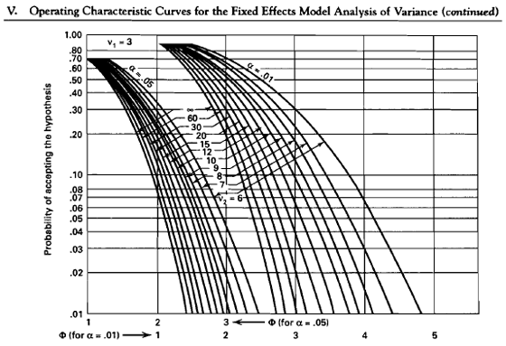
The OC curves for the fixed effects model are given in the Appendix V.
The usual way to use these charts is to define the difference in the means, \(\delta = \text{max}(\mu_i) - \text{min}(\mu_i)\), that you want to detect, specify the value of \(\sigma^2\), and then for the LFC use :
\(\Phi^2=\dfrac{n\delta^2}{2a\sigma^2}\)
for various values of n. The Appendix V gives \(\beta\), where \(1 - \beta\) is the power for the test where \(\nu_1 = a - 1\) and \(\nu_2 = a(n - 1)\). Thus after setting n, you must calculate \(\nu_1\) and \(\nu_2\) to use the table.
Example: We consider an \(\alpha = 0.05\) level test for \(a = 4\) using \(\delta = 10\) and \(\sigma^2 = 144\) and we want to find the sample size n to obtain a test with power = 0.9.
Let's guess at what our n is and see how this work. Say we let n be equal to 20, let \(\delta = 10\), and \(\sigma = 12\) then we can calculate the power using Appendix V. Plugging in these values to find \(\Phi\) we get \(\Phi = 1.3\).

Now go to the chart where \(\nu_2\) is 80 - 4 = 76 and \(\Phi = 1.3\). This gives us a Type II error of \(\beta = 0.45\) and \(\text{power} = 1 - \beta = 0.55\).
It seems that we need a larger sample size.
Well, let's use a sample size of 30. In this case we get \(\Phi^2 = 2.604\), so \(\Phi = 1.6\).
Now with \(\nu_2\) a bit more at 116, we have \(\beta = 0.30\) and power = 0.70.
So we need a bit more than n = 30 per group to achieve a test with power = 0.8.
Review the video below for a 'walk-through' this procedure using Appendix V in the back of the text.