Lesson 5: Introduction to Factorial Designs
Lesson 5: Introduction to Factorial DesignsIntroduction
Factorial designs are the basis for another important principle besides blocking - examining several factors simultaneously. We will start by looking at just two factors and then generalize to more than two factors. Investigating multiple factors in the same design automatically gives us replication for each of the factors.
Objectives
- Factorial Designs as among the most common experimental designs
- Two factor Factorial Design and its extension to the General Factorial Designs
- Sample size determination in Factorial Designs
5.1 - Factorial Designs with Two Treatment Factors
5.1 - Factorial Designs with Two Treatment FactorsFor now we will just consider two treatment factors of interest. It looks almost the same as the randomized block design model only now we are including an interaction term:
\(Y_{ijk} = \mu + \alpha_i + \beta_j + (\alpha\beta)_{ij} + e_{ijk}\)
where \(i = 1, \dots, a, j = 1, \dots, b, \text{ and } k = 1, \dots, n\). Thus we have two factors in a factorial structure with n observations per cell. As usual, we assume the \(e_{ijk} ∼ N(0, \sigma^2)\), i.e. independently and identically distributed with the normal distribution. Although it looks like a multiplication, the interaction term need not imply multiplicative interaction.
The Effects Model vs. the Means Model
The cell means model is written:
\(Y_{ijk}=\mu_{ij} + e_{ijk}\)
Here the cell means are: \(\mu_{11}, \dots , \mu_{1b}, \dots , \mu_{a1} \dots \mu_{ab}\). Therefore we have a × b cell means, μij. We will define our marginal means as the simple average over our cell means as shown below:
\(\bar{\mu}_{i.}=\frac{1}{b} \sum\limits_j \mu_{ij}\), \(\bar{\mu}_{.j}=\frac{1}{a} \sum\limits_i \mu_{ij}\)
From the cell means structure we can talk about marginal means and row and column means. But first we want to look at the effects model and define more carefully what the interactions are We can write the cell means in terms of the full effects model:
\(\mu_{ij} = \mu + \alpha_i + \beta_j + (\alpha\beta)_{ij}\)
It follows that the interaction terms \((\alpha \beta)_{ij}\)are defined as the difference between our cell means and the additive portion of the model:
\((\alpha\beta)_{ij} = \mu_{ij} - (\mu + \alpha_i + \beta_j) \)
If the true model structure is additive then the interaction terms\((\alpha \beta)_{ij}\) are equal to zero. Then we can say that the true cell means, \(\mu_{ij} = (\mu + \alpha_i + \beta_j)\), have additive structure.
Example 1
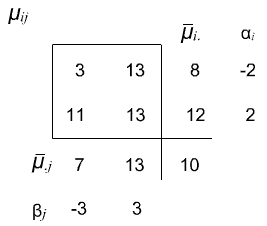
Let's illustrate this by considering the true means \(\mu_{ij} \colon\)
| B | |||||||
|---|---|---|---|---|---|---|---|
| \(\mu_{ij}\) | |||||||
| A | 1 | 2 | \(\bar{\mu}_{i.}\) | \(\alpha_i\) | |||
| 1 | 5 | 11 | 8 | -2 | |||
| 2 | 9 | 15 | 12 | 2 | |||
| \(\bar{\mu}_{.j}\) | 7 | 13 | 10 | ||||
| \(\beta_j\) | -3 | 3 | |||||
Note that both a and b are 2, thus our marginal row means are 8 and 12, and our marginal column means are 7 and 13. Next, let's calculate the \(\alpha\) and the \(\beta\) effects; since the overall mean is 10, our \(\alpha\) effects are -2 and 2 (which sum to 0), and our \(\beta\) effects are -3 and 3 (which also sum to 0). If you plot the cell means you get two lines that are parallel.
The difference between the two means at the first \(\beta\) factor level is 9 - 5 = 4. The difference between the means for the second \(\beta\) factor level is 15 - 11 = 4. We can say that the effect of \(\alpha\) at the first level of \(\beta\) is the same as the effect of \(\alpha\) at the second level of \(\beta\). Therefore we say that there is no interaction and as we will see the interaction terms are equal to 0.
This example simply illustrates that the cell means, in this case, have additive structure. A problem with data that we actually look at is that you do not know in advance whether the effects are additive or not. Because of random error, the interaction terms are seldom exactly zero. You may be involved in a situation that is either additive or non-additive, and the first task is to decide between them.
Now consider the non-additive case. We illustrate this with Example 2 which follows.
Example 5.2
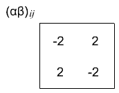
This example was constructed so that the marginal means and the overall means are the same as in Example 1. However, it does not have additive structure.

Using the definition of interaction:
\((\alpha \beta)_{ij} = \mu_{ij} - (\mu + \alpha_i + \beta_j)\)
which gives us \((\alpha \beta)_{ij}\) interaction terms that are -2, 2, 2, -2. Again, by the definition of our interaction effects, these \((\alpha \beta)_{ij}\) terms should sum to zero in both directions.

We generally call the \(\alpha_i\) terms the treatment effects for treatment factor A and the \(\beta_j\) terms for treatment factor B, and the \((\alpha \beta)_{ij}\) terms the interaction effects.
The model we have written gives us a way to represent in a mathematical form a two-factor design, whether we use the means model or the effects model, i.e.,
\(Y_{ijk} = \mu_{ij} + e_{ijk}\)
or
\(Y_{ijk} = \mu + \alpha_i + \beta_j + (\alpha\beta)_{ij} + e_{ijk}\)
There is really no benefit to the effects model when there is interaction, except that it gives us a mechanism for partitioning the variation due to the two treatments and their interactions. Both models have the same number of distinct parameters. However, when there is no interaction then we can remove the interaction terms from the model and use the reduced additive model.
Now, we'll take a look at the strategy for deciding whether our model fits, whether the assumptions are satisfied and then decide whether we can go forward with an interaction model or an additive model. This is the first decision. When you can eliminate the interactions because they are not significantly different from zero, then you can use the simpler additive model. This should be the goal whenever possible because then you have fewer parameters to estimate, and a simpler structure to represent the underlying scientific process.
Before we get to the analysis, however, we want to introduce another definition of effects - rather than defining the \(\alpha_i\) effects as deviation from the mean, we can look at the difference between the high and the low levels of factor A. These are two different definitions of effects that will be introduced and discussed in this chapter and the next, the \(\alpha_i\) effects and the difference between the high and low levels, which we will generally denote as the A effect.
Factorial Designs with 2 Treatment Factors, cont'd
For a completely randomized design, which is what we discussed for the one-way ANOVA, we need to have n × a × b = N total experimental units available. We randomly assign n of those experimental units to each of the a × b treatment combinations. For the moment we will only consider the model with fixed effects and constant experimental random error.
The model is:
\(Y_{ijk} = \mu + \alpha_i + \beta_j + (\alpha\beta)_{ij} + e_{ijk}\)
\(i = 1, \dots , a\)
\(j = 1, \dots , b\)
\(k = 1, \dots , n\)
Read the text section 5.3.2 for the definitions of the means and the sum of squares.
Testing Hypotheses
We can test the hypotheses that the marginal means are all equal, or in terms of the definition of our effects that the \(\alpha_i\)'s are all equal to zero, and the hypothesis that the \(\beta_j\)'s are all equal to zero. And, we can test the hypothesis that the interaction effects are all equal to zero. The alternative hypotheses are that at least one of those effects is not equal to zero.
How we do this, in what order, and how do we interpret these tests?
One of the purposes of a factorial design is to be efficient about estimating and testing factors A and B in a single experiment. Often we are primarily interested in the main effects. Sometimes, we are also interested in knowing whether the factors interact. In either case, the first test we should do is the test on the interaction effects.
The Test of H0: \((\alpha\beta)_{ij}=0\)
If there is interaction and it is significant, i.e. the p-value is less than your chosen cut off, then what do we do? If the interaction term is significant that tells us that the effect of A is different at each level of B. Or you can say it the other way, the effect of B differs at each level of A. Therefore, when we have significant interaction, it is not very sensible to even be talking about the main effect of A and B, because these change depending on the level of the other factor. If the interaction is significant then we want to estimate and focus our attention on the cell means. If the interaction is not significant, then we can test the main effects and focus on the main effect means.
The estimates of the interaction and main effects are given in the text in section 5.3.4.
Note that the estimates of the marginal means for A are the marginal means:
\(\bar{y}_{i..}=\dfrac{1}{bn} \sum\limits_j \sum\limits_k y_{ijk}\), with \(var(\bar{y}_{i..})=\dfrac{\sigma^2}{bn}\)
A similar formula holds for factor B, with
\(var(\bar{y}_{.j.})=\dfrac{\sigma^2}{an}\)
Just the form of these variances tells us something about the efficiency of the two-factor design. A benefit of a two factor design is that the marginal means have n × b number of replicates for factor A and n × a for factor B. The factorial structure, when you do not have interactions, gives us the efficiency benefit of having additional replication, the number of observations per cell times the number of levels of the other factor. This benefit arises from factorial experiments rather than single factor experiments with n observations per cell. An alternative design choice could have been to do two one-way experiments, one with a treatments and the other with b treatments, with n observations per cell. However, these two experiments would not have provided the same level of precision, nor the ability to test for interactions.
Another practical question: If the interaction test is not significant what should we do?
Do we get remove the interaction term in the model? You might consider dropping that term from the model. If n is very small and your df for error are small, then this may be a critical issue. There is a 'rule of thumb' that I sometimes use in these cases. If the p-value for the interaction test is greater than 0.25 then you can drop the interaction term. This is not an exact cut off but a general rule. Remember, if you drop the interaction term, then a variation accounted for by SSab would become part of the error and increasing the SSE, however your error df would also become larger in some cases enough to increase the power of the tests for the main effects. Statistical theory shows that in general dropping the interaction term increases your false rejection rate for subsequent tests. Hence we usually do not drop nonsignificant terms when there are adequate sample sizes. However, if we are doing an independent experiment with the same factors we might not include interaction in the model for that experiment.
What if n = 1, and we have only 1 observation per cell? If n = 1 then we have 0 df for SSerror and we cannot estimate the error variance with MSE. What should we do in order to test our hypothesis? We obviously cannot perform the test for interaction because we have no error term.
If you are willing to assume, and if it is true that there is no interaction, then you can use the interaction as your F-test denominator for testing the main effects. It is a fairly safe and conservative thing to do. If it is not true then the MSab will tend to be larger than it should be, so the F-test is conservative. You're not likely to reject a main effect if it is not true. You won't make a Type I error, however you could more likely make a Type II error.
Extension to a 3 Factor Model
The factorial model with three factors can be written as:
\(Y_{ijk} = \mu + \alpha_i + \beta_j + \gamma_k + (\alpha \beta)_{ij} + (\alpha \gamma)_{ik} + (\beta \gamma)_{jk} + (\alpha \beta \gamma)_{ijk} + e_{ijkl}\)
where \(i = 1, \dots , a, j = 1 , \dots , b, k = 1 , \dots , c, l = 1 , \dots , n\)
We extend the model in the same way. Our analysis of variance has three main effects, three two-way interactions, a three-way interaction and error. If this were conducted as a Completely Randomized Design experiment, each of the a × b × c treatment combinations would be randomly assigned to n of the experimental units.
Sample Size Determination [Section 5.3.5]
We first consider the two-factor case where N = a × b × n, (n = the number of replicates per cell). The non-centrality parameter for calculating sample size for the A factor is:
\(\phi^2 = ( nb \times D^{2}) / ( 2a \times \sigma^2)\)
where D is the difference between the maximum of \(\bar{\mu_{i.}}\) and the minimum of \(\bar{\mu_{i.}}\), and where b is the number of observations in each level of factor A.
Actually, at the beginning of our design process, we should decide how many observations we should take, if we want to find a difference of D, between the maximum and the minimum of the true means for the factor A. There is a similar equation for factor B.
\(\phi^{2} = ( na \times D^{2} ) / ( 2b \times \sigma^{2})\)
where na is the number of observations in each level of factor B.
In the two factor case, this is just an extension of what we did in the one-factor case. But now we have the marginal means benefiting from a number of observations per cell and the number of levels of the other factor. In this case, we have n observations per cell, and we have b cells. So, we have nb observations.
5.2 - Another Factorial Design Example - Cloth Dyes
5.2 - Another Factorial Design Example - Cloth DyesMinitab®
Consider the cloth dyes data from Problem 5.19 in the text:
For each combination of time, temperature and operator, there are three observations. Now we have a case where there are three factors and three observations per cell. Let's run this model in Minitab.
General Linear Model: Score versus Temperature, Cycle Time, Operator
| Factor | Type | Levels | Values |
|---|---|---|---|
| Temperature | fixed | 2 | 300, 350 |
| Cycle Time | fixed | 3 | 40, 50, 60 |
| Operator | fixed | 3 | 1, 2, 3 |
Analysis of Variance for Score, using Adjusted SS for Tests
| Source | DF | Seq SS | Adj SS | Adj MS | F | P |
|---|---|---|---|---|---|---|
| Temperature | 1 | 50.074 | 50.074 | 50.074 | 15.28 | 0.000 |
| Cycle Time | 2 | 436.000 | 436.000 | 218.000 | 66.51 | 0.000 |
| Operator | 2 | 261.333 | 261.333 | 130.667 | 39.86 | 0.000 |
| Temperature*Cycle Time | 2 | 78.815 | 78.815 | 39.407 | 12.02 | 0.000 |
| Temperature*Operator | 2 | 11.259 | 11.259 | 5.630 | 1.72 | 0.194 |
| Cycle Time*Operator | 4 | 355.667 | 355.667 | 88.917 | 27.13 | 0.000 |
| Temperature*Cycle Time*Operator | 4 | 46.185 | 46.185 | 11.546 | 3.52 | 0.016 |
| Error | 36 | 118.000 | 118.000 | 3.278 | ||
| Total | 53 | 1357.333 | ||||
| S = 1.81046 R-Sq = 91.31% R-Sq(adj) = 87.20% | ||||||
Unusual Observations for Score
| Obs | Score | Fit | SE Fit | Residual | St Resid |
|---|---|---|---|---|---|
| 5 | 34.0000 | 37.0000 | 1.0453 | -3.0000 | -2.03 R |
| 46 | 28.0000 | 25.0000 | 1.0453 | 3.0000 | 2.03 R |
| R denotes an observation with a large standardized residual. | |||||
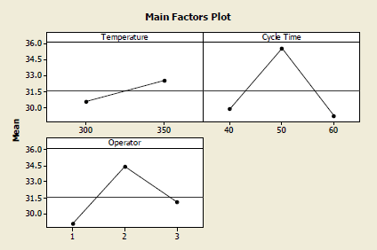
The ANOVA table shows us that the main effects due to cycle time, operator, and temperature are all significant. The two-way interactions for cycle time by operator and cycle time by temperature are significant. But the operator by temperature is not significant but the dreaded three-way interaction is significant. What does it mean when a three-way interaction is significant?
Let's take a look at the factor plots:


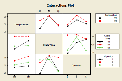
These interaction plots show us the three sets of two-way cell means, each of the three are plotted in two different ways. This is a useful plot to try to understand what is going on. These are all the two-way plots.
Typically a three-way interaction would be plotted as two panels... showing how the two-way interactions differ across the levels of the third factor. Minitab does not do that for you automatically.
Let's think about how this experiment was done. There are three observations for each combination of factors. Are they actually separate experimental units or are they simply three measurements on the same experimental unit? If they are simply three measurements on the same piece of cloth that was all done in the same batch, for instance, then they are not really independent. If this is the case, then another way to look at this data would be to average those replications. In this case there is only 1 observation for each treatment, so that there would be no d.f. for error. However, the way the problem is presented in the text, they appear to have been treated independently and thus are true replicates, leading to 36 d.f. for error.
You could also think about the operator not as a factor that you're interested in but more as a block factor, i.e. a source of variation that we want to remove from the study. What we're really interested in is the effect of temperature and time on the process of dyeing the cloth. In this case we could think about using the operator as a block effect. Running the analysis again, now we get the same plot but look at the ANOVA table: now the interactions related to operator have been pooled as a part of the error. So the residual error term now has 2 + 4 + 4 + 36 = 46 df for error. Note also that if you do use the operator as a treatment factor, it probably should be considered random. In this case, you would probably want to consider the 2 and 3-way interactions involving operator to be random effects. Experiments in which some factors are fixed and others are random are called mixed effects experiments. The analysis of mixed effects experiments is discussed in Chapter 13.
General Linear Model: Score versus Temperature, Cycle Time, Operator
| Factor | Type | Levels | Values |
|---|---|---|---|
| Temperature | fixed | 2 | 300, 350 |
| Cycle Time | fixed | 3 | 40, 50, 60 |
| Operator | fixed | 3 | 1, 2, 3 |
Analysis of Variance for Score, using Adjusted SS for Tests
| Source | DF | Seq SS | Adj SS | Adj MS | F | P |
|---|---|---|---|---|---|---|
| Temperature | 1 | 50.07 | 50.07 | 50.07 | 4.34 | 0.043 |
| Cycle Time | 2 | 436.00 | 436.00 | 218.00 | 18.88 | 0.000 |
| Operator | 2 | 261.33 | 261.33 | 130.67 | 11.32 | 0.000 |
| Temperature*Cycle Time | 2 | 78.81 | 78.81 | 39.41 | 11.32 | 0.041 |
| Error | 46 | 531.11 | 531.11 | 11.55 | ||
| Total | 53 | 1357.33 | ||||
| S = 3.39792 R-Sq = 60.87% R-Sq(adj) = 54.92% | ||||||
Unusual Observations for Score
| Obs | Score | Fit | SE Fit | Residual | St Resid |
|---|---|---|---|---|---|
| 28 | 23.0000 | 30.1111 | 1.3079 | -7.1111 | -2.27 R |
| 48 | 39.0000 | 32.1111 | 1.3079 | 6.8889 | 2.20 R |
| R denotes an observation with a large standardized residual. | |||||
What this points out is the importance of distinguishing what is a block factor, and which are the treatment factors when you have a multifactor experimental design. This should be apparent from how the experiment was conducted, but if the data are already collected when you are introduced to the problem, you need to inquire carefully to understand how the experiment was actually conducted to know what model to use in the analysis.
Let's take a look two examples using this same dataset using Minitab v19. First we will analyze the quantitative factors involved, Cycle Time and Temperature and as though they were qualitative - simply nominal factors.
Next, using Operator as a block we will now use Minitab v19 to treat the quantitative factors as qualitative factors and apply these in a regression analysis.