Lesson 8: 2-level Fractional Factorial Designs
Lesson 8: 2-level Fractional Factorial DesignsOverview
What we did in the last chapter is consider just one replicate of a full factorial design and run it in blocks. The treatment combinations in each block of a full factorial can be thought of as a fraction of the full factorial.
In setting up the blocks within the experiment we have been picking the effects we know would be confounded and then using these to determine the layout of the blocks.
We begin with a simple example.
In an example where we have \(k = 3\) treatments factors with \(2^3 = 8\) runs, we select \(2^p = 2 \text{blocks}\), and use the 3-way interaction ABC to confound with blocks and to generate the following design.
| trt | A | B | C | AB | AC | BC | ABC | I |
|---|---|---|---|---|---|---|---|---|
| (1) | - | - | - | - | ||||
| a | + | - | - | + | ||||
| b | - | + | - | + | ||||
| ab | + | + | - | - | ||||
| c | - | - | + | + | ||||
| ac | + | - | + | - | ||||
| bc | - | + | + | - | ||||
| abc | + | + | + | + |
Here are the two blocks that result using the ABC as the generator:
| Block | 1 | 2 |
|---|---|---|
| ABC | - | + |
| (1) | a | |
| ab | b | |
| ac | c | |
| bc | abc |
A fractional factorial design is useful when we can't afford even one full replicate of the full factorial design. In a typical situation our total number of runs is \(N = 2^{k-p}\), which is a fraction of the total number of treatments.
Using our example above, where \(k = 3\), \(p = 1\), therefore, \(N = 2^2 = 4\)
So, in this case, either one of these blocks above is a one half fraction of a \(2^3\) design. Just as in the block designs where we had AB confounded with blocks - where we were not able to say anything about AB. Now, where ABC is confounded in the fractional factorial we can not say anything about the ABC interaction.
Let's take a look at the first block which is a half fraction of the full design. ABC is the generator of the 1/2 fraction of the \(2^3\) design. Now, take just the fraction of the full design where ABC = -1 and we place it within its own table:
| trt | A | B | C | AB | AC | BC | ABC | I |
|---|---|---|---|---|---|---|---|---|
| (1) | - | - | - | + | + | + | - | + |
| ab | + | + | - | + | - | - | - | + |
| ac | + | - | + | - | + | - | - | + |
| bc | - | + | + | - | - | + | - | + |
Notice the contrast defining the main effects (similar colors) - there is an aliasing of these effects. Notice that columns with the same color are just -1 times one another.
In this half fraction of the design we have 4 observations, therefore we have 3 degrees of freedom to estimate. The degrees of freedom estimate the following effects: A - BC, B - AC, and C - AB. Thus, this design is only useful if the 2-way interactions are not important, since the effects we can estimate are the combined effect of main effects and 2-way interactions.
This is referred to as a Resolution III Design. It is called a Resolution III Design because the generator ABC has three letters, but the properties of this design and all Resolution III designs are such that the main effects are confounded with 2-way interactions.
Let's take a look at how this is handled in Minitab:
Objectives
- Understanding the application of Fractional Factorial designs, one of the most important designs for screening
- Becoming familiar with the terms “design generator”, “alias structure” and “design resolution”
- Knowing how to analyze fractional factorial designs in which there aren’t normally enough degrees of freedom for error
- Becoming familiar with the concept of “foldover” either on all factors or on a single factor and application of each case
- Being introduced to “Plackett-Burman Designs” as another class of major screening designs
8.1 - More Fractional Factorial Designs
8.1 - More Fractional Factorial DesignsWe started our discussion with a single replicate of a factorial design. Then we squeezed it into blocks, whether it was replicated or not. Now we are going to construct even more sparse designs. There will be a large number of factors, k, but the total number of observations will be \(N = 2^{k-p}\), so we keep the total number of observations relatively small as k gets large.
The goal is to create designs that allow us to screen a large number of factors but without having a very large experiment. In the context where we are screening a large number of factors, we are operating under the assumption that only a few are very important. This is called sparsity of effects. We want an efficient way to screen the large number of factors knowing in advance that there will likely be only two or three factors that will be the most important ones. Hopefully, we can detect those factors even with a relatively small experiment.
We started this chapter by looking at the \(2^{3-1}\) fractional factorial design. This only has four observations. This is totally unrealistic but served its purpose in illustrating how this design works. ABC was the generator, which is equal to the Identity, (I = ABC or I = -ABC). This defines the generator of the design and from this we can determine which effects are confounded or aliased with which other effects
Let's use the concept of the generator and construct a design for the \(2^{4-1}\) fractional factorial. This gives us a one half fraction of the \(2^4\) design. Again, we want to pick a high order interaction. Let's select ABCD as the generator (I = ABCD) and by hand we can construct the design. I = ABCD implies that D = ABC. First of all, \(2^{4-1} = 2^3 = 8\). So, we will have eight observations in our design. Here is a basic \(2^3\) design in standard Yates notation defined by the levels of A, B, and C:
| trt | A | B | C | D = ABC |
|---|---|---|---|---|
| (1) | - | - | - | - |
| a | + | - | - | + |
| b | - | + | - | + |
| ab | + | + | - | - |
| c | - | - | + | + |
| ac | + | - | + | - |
| bc | - | + | + | - |
| abc | + | + | + | + |
We can then construct the levels of D by using the relationship where D = ABC. Therefore, in the first row where all the treatments are minus, D = -1*-1*-1 = -1. In the second row, +1, and so forth. As before we write - and + as a shorthand for -1 and +1.
This is a one half fraction of the \(2^4\) design. A full \(2^4\) design would have 16 factors.
This \(2^{4-1} \)design is a Resolution IV design. The resolution of the design is based on the number of the letters in the generator. If the generator is a four letter word, the design is Resolution IV. The number of letters in the generator determines the confounding or aliasing properties in the resulting design.
We can see this best by looking at the expression I = ABCD. We obtain the alias structure by multiplying \(A \times I = A \times ABCD = A^{2}BCD\) which implies \(A = BCD\). If we look at the aliasing that occurs we would see that A is aliased with BCD, and similarly all of the main effects are aliased with a three-way interaction:
\(B = ACD\)
\(C = ABD\)
\(D = ABC\)
Main effects are aliased with three-way interactions. Using the same process, we see that two-way interactions are aliased with other two-way interactions:
\(AB = CD\)
\(AC = BD\)
\(AD = BC\)
In total, we have seven effects, the number of degrees of freedom in this design. The only effects that are estimable from this design are the four main effects assuming the 3-way interactions are zero and the three 2-way interactions that are confounded with other 2-way interactions. All 16 effects are accounted for with these seven contrasts plus the overall mean.
Let's take a look at how this type of design is generated in Minitab...
Resolution IV Designs
What you need to know about Resolution IV designs:
- the main effects are aliased with the 3-way interactions. This is just the result of the fact that this is a four letter effect that we are using as the generator.
- the 2-way interactions are aliased with each other. Therefore, we can not determine from this type of design which of the 2-way interactions are important because they are confounded or aliased with each other.
Resolution IV designs are preferred over Resolution III designs. Resolution III designs do not have as good properties because main effects are aliased with two-way interactions. Again, we work from the assumption that the higher order interactions are not as important. We want to keep our main effects clear of other important effects.
The 5 Factor Design
Here we let \(k = 5\) and \(p = 1\), again, so that we have a one half fraction of a \(2^5\) design. Now we have five factors, A, B, C, D and E, each at two levels. What would we use as our generator? Since we are only picking one generator, we should choose the highest order interaction as possible. So we will choose I = ABCDE, the five-way interaction.
Let's use Minitab to set this up. Minitab gives us a choice of a one half or one-fourth fraction. We will select the one-half fraction. It says it is a Resolution V design because it has a five letter generator I = ABCDE or (E = ABCD).
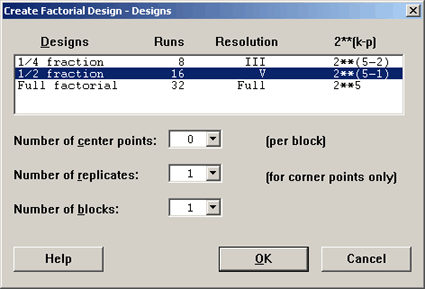
We get a \(2^{5-1}\), so there are 16 observations. Taking a look at the design:
Fractional Factorial Design
| Factors: | 5 | Base Design: | 5, 16 | Resolution: | V |
| Runs: | 16 | Replicates: | 1 | Fraction: | 1/2 |
| Blocks: | 1 | Center pts (total): | 0 | ||
Design Generators: E = ABCD
Alias Structure
I + ABCDE
A + BCDE
B + ACDE
C + ABDE
D + ABCE
E + ABCD
AB + CDE
AC + BDE
AD + BCE
AE + BCD
BC + ADE
BD + ACE
BE + ACD
CD + ABE
CE + ABD
DE + ABC
E = ABCD gives us the basis for the resolution of the design.
Let's look at the properties of a Resolution V design. We can see that:
- the main effects are 'clear' of 2-way and 3-way interactions.
- the main effects are only confounded with 4-way interactions or higher, so this gives us really good information, and
- the 2-way interactions are 'clear' of each other but are aliased with 3-way interactions.
The Resolution V designs are everybody's favorite because you can estimate main effects and two-way interactions if you are willing to assume that three-way interactions and higher are not important.
You can go higher, with Resolution VI, VII etc. designs, however, Resolution III is more or less the minimum, and Resolution IV and V are increasing in good properties in terms of being able to estimate the effects.
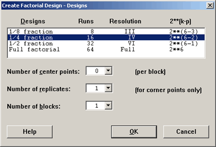
A One-Fourth Fractional Design, or a \(\frac{1}{2}^2\) Fraction of a \(2^k\) design
Let's try to construct a 1/4 fractional design using the previous example where \(k = 4\) factors. In this case \(p = 2\), therefore we will have to pick 2 generators in order to construct this type of design.
As in the previous example \(k = 4\), but now \(p = 2\), so this would give us \(2^{4 -2} = 4\) observations. A problem that we can foresee here is that we only have a total of 3 degrees of freedom to estimate. But we have four main effects, so a main effect is going to have to be confounded or aliased with another main effect. Hence, this design is not even a Resolution III. Let's go ahead anyway.
Let's pick ABCD, as we did before, as one generator and ABC as the other. So we would have ABCD × ABC = D as our third generator.
This is not good ... now we have a main effect as a generator which means the main effect would be confounded with the mean .... we can do better than that.
Let's pick ABCD and then AB as a second generator, this would give us ABCD × AB = CD as our third generator. We pick two but we must also include a generalized interaction.
Now the smallest word in our generator set is a two letter word - so this means that this is a Resolution II design. But we found out that a Resolution II designs tell us that the main effects are aliased with each other, ... hence not a good design if we want to learn which main effects are important.
Let's try another example...
Let's say we have \(k = 5\) and \(p = 2\). We have five factors, so again we need to pick two generators. We want to pick the generators so that the generators and their interactions are each as large a word as possible. This is very similar to what we were doing when we were confounding in blocks.
Let's pick the 4-way interaction ABCD, and CDE. Then the generalized interaction is \(ABCD \times CDE = ABE\). In this case, in the way we picked them the smallest number of letters is 3 so this is a Resolution III design.
We can construct this design in the same way we had previously. We begin with \(2^{5-2} = 2^{3} = 8\) observations which are constructed from all combinations of A, B, and C, then we'll use our generators to define D and E. Note that I = ABCD tells us that D = ABC, and the other generator I = CDE tells us that E = CD. Now we can define the new columns D = ABC and E = CD. Although D and E weren't a part of the original design, we were able to construct them from the two generators as shown below:
| trt | A | B | C | D = ABC | E = CD |
|---|---|---|---|---|---|
| (1) | - | - | - | - | + |
| a | + | - | - | + | - |
| b | - | + | - | + | - |
| ab | + | + | - | - | + |
| c | - | - | + | + | + |
| ac | + | - | + | - | - |
| bc | - | + | + | - | - |
| abc | + | + | + | + | + |
Now we have a design with eight observations, \(2^3\), with five factors. Our generator set is: I = ABCD = CDE = ABE. This is a Resolution III design because the smallest word in the generator set has only three letters. Let's look at this in Minitab ...
Example: Resolution IV Design
Let's take \(k = 6\) and \(p = 2\), now we again have to choose two generators with the highest order possible, such that the generalized interaction is also as high as possible. We have factors A, B, C, D, E and F to choose from. What should we choose as generators?
Let's try ABCD and CDEF. The generalized interaction of these two = ABEF. We have strategically chosen two four letter generators whose generalized interaction is also four letters. This is the best that we can do. This results in a \(2^{6-2}\) design, which is sometimes written like this, \(2^{6-2}_{IV}\), because it is a Resolution IV design.
In Minitab we can see the available designs for six factors in the table below:
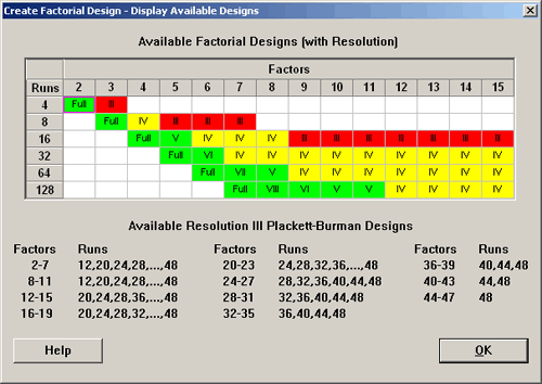
... with six factors, a \(2^{6-2} = 2^{4}\) design, which has 16 observations, is located in the six factor column, the 16 observation row. This tells us that this design is a Resolution IV, (in yellow). We know from this table that this type of design exists, so in Minitab we can specify this design.
... which results in the following output.
Fractional Factorial Design
| Factors: | 6 | Base Design: | 6, 16 | Resolution: | IV |
| Runs: | 16 | Replicates: | 1 | Fraction: | 1/4 |
| Blocks: | 1 | Center pts (total): | 0 | ||
Design Generators: E = ABC, F = BCD
Alias Structure
I + ABCE + ADEF + BCDF
A + BCE + DEF + ABCDF
B + ACE + CDF + ABDEF
C + ABE + BDF + ACDEF
D + AEF + BCF + ABCDE
E + ABC + ADF + BCDEF
F + ADE + BCD + ABCEF
AB + CE + ACDF + BDEF
AC + BE + ABDF + CDEF
AD + EF + ABCF + BCDE
AE + BC + DF + ABCDEF
AF + DE + ABCD + BCEF
BD + CF + ABEF + ACDE
BF + CD + ABDE + ACEF
ABD + ACF + BEF + CDE
ABF + ACD + BDE + CEF
In Minitab by default ABCE and BCDF were chosen as the design generators. The design was constructed by starting with the full factorial of factors A, B, C, and D. Minitab then generated E by using the first three columns, A, B and C. Then it could choose F = BCD.
Because the generator set, \(I = ABCE = ADEF = BCDF\), contains only four letter words, this is classified as a Resolution IV design. All the main effects are confounded with 3-way interactions and a 5-way interaction. The 2-way interactions are aliased with each other. Again, this describes the property of the Resolution IV design.
8.2 - Analyzing a Fractional Factorial Design
8.2 - Analyzing a Fractional Factorial DesignWe discussed designing experiments, but now let's discuss how we would analyze these experiments. We take an example we saw before. The response Y is filtration rate in a chemical pilot plant and the four factors are: A = temperature, B = pressure, C = concentration and D = stirring rate. (Example 2 from Chapter 6, Ex6-2.mwx | Ex6-2.csv)
This experimental design has 16 observations, a \(2^4\) with one complete replicate. This is the example we looked at with one observation per cell when we introduced a normal scores plot.
Our final model ended up with three factors, A, C and D, and two of their interactions, AC and AD. This was based on one complete replicate of this design. What might we have learned if we had done an experiment half this size, N = 8? If we look at the fractional factorial - one half of this design - where we have D = ABC or I = ABCD as the generator - this creates a design with 8 observations.
Fractional Factorial Design
| Factors: | 4 | Base Design: | 4, 8 | Resolution: | IV |
| Runs: | 8 | Replicates: | 1 | Fraction: | 1/2 |
| Blocks: | 1 | Center pts (total): | 0 | ||
Design Generators: D = ABC
Alias Structure
I + ABCD
A + BCD
B + ACD
C + ABD
D + ABC
AB + CD
AC + BD
AD + BC
The alias structure is a four letter word, therefore this is a Resolution IV design, A, B, C and D are each aliased with a 3-way interaction, (so we can't estimate them any longer), and the two way interactions are aliased with each other.
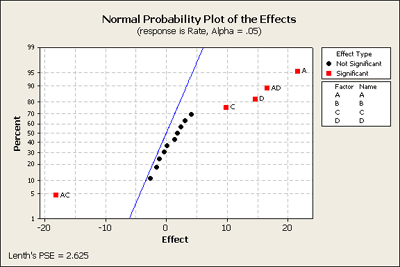
If we look at the analysis of this 1/2 fractional factorial design and we put all of the terms in the model, (of course some of these are aliased with each other), and we will look at the normal scores plot. What do we get? (The data are in Ex6_2Half.MTW)
We only get seven effects plotted, since there were eight observations. The overall mean does not show up here. These points are labeled but because there are only seven of them there is no estimate of error. Let's look at another plot that we haven't used that much yet - the Pareto plot. This type of plot looks at the effects and orders them from largest to smallest showing you the relative sizes of the effects. Although we do not know what is significant and what is not significant, this still might be a helpful plot to look at to better understand the data.
This Pareto plot shows us that the three main effects A, C, and D that were most significant in the full design are still important as well as the two interactions, AD and AC. However, B and AB are clearly not as large. (You can do this using the Stat > DOE > Factorial > Analyze and click on Graph.)
What can we learn from this? Let's try to fit a reduced model from the information that we gleaned from this first step. We will include all the main effects and the AC and AD interactions.
In the analysis, we have four main effects ...
Factorial Fit: Y-Rate versus A, B, C, D
Estimated Effects and Coefficients for Y-Rate (coded units)
| Term | Effect | Coef | SE Coef | T | P |
|---|---|---|---|---|---|
| Constant | 70.750 | 0.5000 | 141.50 | 0.004 | |
| A | 19.000 | 9.500 | 0.5000 | 19.00 | 0.033 |
| B | 1.500 | 0.750 | 0.5000 | 1.50 | 0.374 |
| C | 14.000 | 7.000 | 0.5000 | 14.00 | 0.045 |
| D | 16.500 | 8.250 | 0.5000 | 16.50 | 0.039 |
| A*C | -18.500 | -9.250 | 0.5000 | -18.50 | 0.034 |
| A*D | 19.000 | 9.500 | 0.5000 | 19.00 | 0.033 |
| S = 1.41421 R-Sq = 99.93% R-Sq(adj) = 99.54% | |||||
Analysis of Variance for Y-Rate (coded units)
| Source | DF | Seq SS | Adj SS | Adj MS | F | P |
|---|---|---|---|---|---|---|
| Main Effects | 4 | 1663.00 | 1663.00 | 415.750 | 207.88 | 0.052 |
| 2-Way Interactions | 2 | 1406.50 | 1406.50 | 703.250 | 351.63 | 0.038 |
| Residual Error | 1 | 2.00 | 2.00 | 2.000 | ||
| Total | 7 | 3071.50 | ||||
... overall they are almost significant, (.052), and the overall two-way interactions, (.038) but we only have one degree of freedom of error - so this makes this a very low-power test. However, this is the price that you would pay with a fractional factorial. If we look above at the individual effects, B as we saw on the plot appears to be not important, we have further evidence that we should drop this from the analysis.
Back to Minitab and let's drop the B term because it doesn't show up as a significant main effect nor as part of any of the interactions.
Factorial Fit: Y-Rate versus A, C, D
Estimated Effects and Coefficients for Y-Rate (coded units)
| Term | Effect | Coef | SE Coef | T | P |
|---|---|---|---|---|---|
| Constant | 70.750 | 0.6374 | 111.0 | 0.000 | |
| A | 19.000 | 9.500 | 0.6374 | 14.90 | 0.004 |
| C | 14.000 | 7.000 | 0.6374 | 10.98 | 0.008 |
| D | 16.500 | 8.250 | 0.6374 | 12.94 | 0.006 |
| A*C | -18.500 | -9.250 | 0.6374 | -14.51 | 0.005 |
| A*D | 19.000 | 9.500 | 0.6374 | 14.90 | 0.004 |
| S = 1.80278 R-Sq = 99.79% R-Sq(adj) = 99.26% | |||||
Analysis of Variance for Y-Rate (coded units)
| Source | DF | Seq SS | Adj SS | Adj MS | F | P |
|---|---|---|---|---|---|---|
| Main Effects | 3 | 1658.50 | 1658.50 | 552.833 | 170.10 | 0.006 |
| 2-Way Interactions | 2 | 1406.50 | 1406.50 | 703.250 | 216.38 | 0.005 |
| Residual Error | 2 | 6.50 | 6.50 | 3.250 | ||
| Total | 7 | 3071.50 | ||||
Now the overall main effects and 2-way interactions are significant. Residual error still only has 2 degrees of freedom, but this gives us an estimate at least and we can also look at the individual effects.
So, fractional factorials are useful when you hope or expect that not all of the factors are going to be significant. You are screening for factors to drop out of the study. In this example, we started with a \(2^{4 - 1}\) design but when we dropped B we ended up with a \(2^3\) design with 1 observation per cell.
This is a typical scenario, you begin by screening a large number of factors and end up with a smaller set. We still don't know much about the factors and this is still a pretty thin or weak design but it gives you the information that you need to take the next step. You can now do a more complete experiment on fewer factors.
8.3 - Foldover Designs
8.3 - Foldover DesignsFoldover designs are useful when you are involved in sequentially testing a set of factors. You begin with very small experiments and proceed in stages. We consider this type of design through two examples.
1/8th fractional factorial of a \(2^6\) design
First, we will look at an example with 6 factors and we select a \(2^{6-3}\) design, or a 1/8th fractional factorial of a \(2^6\) design.
In order to select a 1/8 fraction of the full factorial, we will need to choose 3 generators and make sure that the generalized interactions among these three generators are of sufficient size to achieve the higher resolution. In this case it will be a Resolution III as Minitab shows us above.
Let's remind ourselves how we do this. We can choose I = ABD = ACE = BCF as the generators.
Since \(N = 2^{6-3} = 2^3\) observations, we start with a basic \(2^3\) design which would be set up using the following framework. First write down the complete factorial for factors A, B, and C. From that we can generate additional factors based on the available interactions, i.e. we will make D = AB, E = AC, and F = BC. Complete the table below ...
| trt | A | B | C | D = AB | E = AC | F = BC | ABC |
|---|---|---|---|---|---|---|---|
| (1) | - |
-
|
-
|
||||
| a |
+
|
- |
-
|
||||
| b | - | + | - | ||||
| ab |
+
|
+
|
- | ||||
| c | - |
-
|
+ | ||||
| ac |
+
|
- | + | ||||
| bc | - | + |
+
|
||||
| abc |
+
|
+
|
+
|
Our generators are ABD, ACE and BCF. So, our alias structure is created by this equivalence:
I = ABD = ACE = BCF
If these are our generators then all of the generalized interactions among these terms are also part of the generator set. Let's take a look at them:
The 2-way interactions:
- ABD × ACE = BCDE,
- ABD × BCF = ACDF,
- ACE × BCF = ABEF,
and the 3-way interaction:
- ABD × ACE × BCF = DEF
We still have a Resolution III design because the generator set is composed of words, the smallest of which has 3 letters. So you could fill in the framework above for these factors just by multiplying from the basic design, the pluses and minuses.
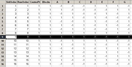
Minitab does this for you. And the worksheet will look like this:
We can estimate all of the main effects and one of the aliased two-way interactions. What this also suggests is that there is one more factor that we could include in a design of this size, N = 8.
1/16th fraction of a \(2^7\) design
Now we consider a 1/16th fraction of a \(2^7\) design or a \(2^{7-4}\) design. Again, we will have only \(N = 2^3 = 8\) observations but now we have seven factors. Thus \(k = 7\) and \(p = 4\).
Let's look at this in Minitab - for seven factors here are the design options ...
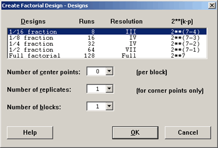
The 1/16 fraction design is a Resolution III design and it is the smallest possible one. Here is what the design looks like:
Fractional Factorial Design
| Factors: | 7 | Base Design: | 7, 8 | Resolution: | III |
| Runs: | 8 | Replicates: | 1 | Fraction: | 1/16 |
| Blocks: | 1 | Center pts (total): | 0 | ||
* NOTE * Some main effects are confounded with two-way interactions.
Design Generators: D = AB, E = AC, F = BC, G = ABC
Alias Structure
I + ABD + ACE + AFG + BCF + BEG + CDG + DEF + ABCG + ABEF + ACDF + ADEG + BCDE + BDFG + CEFG + ABCDEFG
A + BD + CD + FG + BCG + BEF + CDF + DEG + ABCF + ABEG + ACDG + ADEF + ABCDE + ABDFG + ACEFG + BCDEFG
B + AD + CF + EG + ACG + AEF + CDE + DFG + ABCE + ABFG + BCDG + BDEF + ABCDF + ABDEG + GCEFG + ACDEFG
C + AE + BF + DG + ABG + ADF + BDE + EFG + ABCD + ACFG + BCEG + CDEF + ABCEF + ACDEG + BCDFG + ABDEFG
D + AB + CG + EF + ACF + AEG + BCE + BFG + ACDE + ADFG + BCDF + BDEG + ABCDG + ABDEF + CDEFG + ABCEFG
E + AC + BG + DF + ABF + ADG + BCD + CFG + ABDE + AEFG + BCEF + CDEG + ABCEG + ACDEF + BDEFG + ABCDFG
F + AG + BC + DE + ABE + ACD + BDG + CEG + ABDF + ACEF + BEFG + CDFG + ABCFG + ADEFG + BCDEF + ABCDEG
G + AF + BE + CD + ABC + ADE + BDF + CEF + ABDG + ACEG + BCFG + DEFG + ABEFG + ACDFG + BCDEG + ABCDEF
The generators are listed on top. The same first three are as before and then G = ABC, the only one left. The alias structure gets quite convoluted. The reason being that if we were taking a complete replicate of this design, \(2^7\), we could put it into 16 blocks. In this case,we are only looking at one of the 16 blocks in the complete design. In these 16 blocks there are 15 degrees of freedom among these blocks. So, you see I + the 15 effects.
Sometimes people are not interested in seeing all of these higher order interactions after all five-way interactions are not all that interesting. You can clean up this output a bit by using this option found in the 'Results...' dialog box in Minitab:
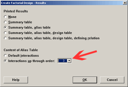
Notice now that the only thing you find in the table are main effects. No 2-way interactions are available. This is a unique design called a Saturated Design. This is the smallest possible design that you could use for 7 factors. Another way to look at this is that for a design with eight observations the maximum number of factors you can include in that design is seven. We are using every degree of freedom to estimate the main effects.
If we moved to the next smallest design where \(N = 16\), then what would the saturated design be? 15 factors. You would have a \(2^{15-11}\), which would give us a \(2^4\) basic design. Then we could estimate up to 15 main effects.
So, you can see with fairly small designs, only 16 observations, we can test for a lot of factors if we are only interested in main effects, using a Resolution III design. Let's see what the options are in Minitab.
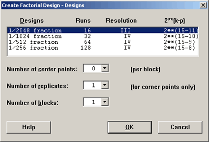
Notice that the largest design shown has 128 runs which is already a very large experiment for 15 factors. You probably wouldn't want more than that.
Folding a Design
We will come back to Saturated designs - but first let's consider the \(2^{7-4}\) design, which is saturated and is a Resolution III design and let's fold it over.
Let's assume we ran this design, we found some interesting effects but we have no degrees of freedom for error.So we want to look at another replicate of this design. Rather than repeating this exact same design we can fold it over.
We can fold it over on all factors, or specify a single factor for folding.
What folding means is to take the design and reverse the sign on all the factors. This would be a fold on all factors.
Now instead of eight observations, we have 16. And if you look at the first eight and compare these with the second set of eight you will see that the signs have simply been reversed.
Look at row 1 and row 9 and you will see that they have the exact opposite signs. Thus you double the basic design with all factors exchanged. Or, you can think of this somewhat as taking one replicate and putting it in blocks, we've now taken two of the blocks to create our design.
These designs are used to learn how to proceed from a basic design, where you might have learned something about one of the factors that looks promising, and you want to give more attention to that factor. This would suggest folding, not on all factors, but folding on that one particular factor. Let's examine why you might want to do this.
In our first example above we started with a Resolution III design, and by folding it over on all factors, we have increased the resolution by one number, in this case it goes from resolution III to IV. So, instead of the main effects being confounded with two-way interactions, which they were before, now they are all clear of the two-way interactions. We still have the two-way interactions confounded with each other however.
Now, let's look at the situation where after the first run we were mostly intrigued by factor B.
Now, rather than fold on all factors we want to fold on just factor B.
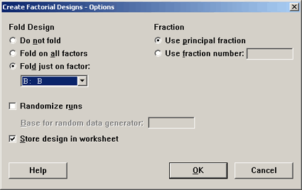
Notice now that in the column for B, the folded part is exactly the opposite. None of the other columns change, just the column for factor B. All of the other columns stayed the same.
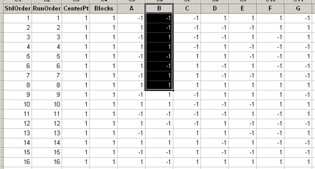
Now look at the alias structure for this design...
Results for: Worksheet 8
| Factors: | 7 | Base Design: | 7, 8 | Resolution: | III |
| Runs: | 16 | Replicates: | 1 | Fraction: | 1/8 |
| Blocks: | 1 | Center pts (total): | 0 | ||
* NOTE * Some main effects are confounded with two-way interactions.
Design Generators: D = AB, E = AC, F = BC, G = ABC
Folded on Factors: B
Alias Structure
I + ACE + AFG + CDG + DEF + ACDF + ADEG + CEFG
A + CE + FG + CDF + DEG + ACDG + ADEF + ACEFG
B + ABCE + ABFG + BCDG + BDEF + ABCDF + ABDEG + BCEFG
C + AE + DG + ADF + EFG + ACFG + CDEF + ACDEG
D + CG + EF + ACF + ACDE + ADFG + CDEFG
E + AC + DF + ADG + CFG + AEFG + CDEG + ACDEF
F + AG + DE + ACD + CEG + ACEF + CDFG + ADEFG
AB + BCE + BFG + BCDF + BDEG + ABCDG + ABDEF + ABCEFG
AD + CF + EG + ACG + AEF + CDE + DFG + ACDEFG
BC + ABE + BDG + ABDF + BEFG + ABCFG + BCDEF + ABCDEG
BD + BCG + BEF + ABCF + ABEG + ABCDE + ABDFG + BCDEFG
BE + ABC + BDF + ABDG + BCFG + ABEFG + BCDEG + ABCDEF
BF + ABG + BDE + ABCD + BCEG + ABCEF + BCDFG + ABDEFG
BG + ABF + BCD + ABDE + BCEF + ABCEG + BDEFG + ABCDFG
ABD + BCF + BEG + ABCG + ABEF + BCDE + BDFG + ABCDEFG
This is still a Resolution III, (we haven't folded on all factors so we don't jump a resolution number). But look at the B factor which we folded. The main effect, B, is aliased with only the four way interactions and higher. Also, notice that all of the 2-way interactions with B are clear of other two-way interactions, so they become estimable. So by only folding on one factor, you get very good information on that factor and its interactions. However, it is still a resolution three design.
There are two purposes for folding; one is taking on another replicate for the purpose of moving to a higher resolution number. The other reason would be to isolate the information on a particular factor. Both of these would be done in the context of doing a sequential experiment, doing an analysis of that and then doing a second stage experiment. If you do this two-stage experiment, performing a second stage based on the first experiment, you should also use stage as the block factor in the analysis.
All of these designs, even though they are fractions of an experiment, should be blocked, if they are done in stages.
One more example ...
Let's go to 8 factors. The minimal design now cannot be eight observations but must be 16. This is a Resolution IV design.
Fractional Factorial Design
| Factors: | 8 | Base Design: | 8, 16 | Resolution: | IV |
| Runs: | 16 | Replicates: | 1 | Fraction: | 1/16 |
| Blocks: | 1 | Center pts (total): | 0 | ||
Design Generators: D = AB, E = AC, F = BC, G = ABC
Alias Structure (up to order 4)
I + ABCG + ABDH + ABEF + ACDF + ACEH + ADEG + AFGH + BCDE + BCFH + BDFG + BEGH + CDGH + CEFG + DEFH
A + BCG + BDH + BEF + CDF + CEH + DEG + FGH
B + ACG + ADH + AEF + CDE + CFH + DFG + EGH
C + ABG + ADF + AEH + BDE + BFH + DFG + EFG
D + ABH + ACF + AEG + BCE + BFG + CGH + EFH
E + ABF + ACH + ADG + BCD + BGH + CFG + DFH
F + ABE + ACD + AGH + BCH + BDG + CEG + DEH
G + ABC + ADE + AFH + BDF + BEH + CDH + CEF
H + ABD + ACE + AFG + BCF + BEG + CDG + DEF
AB + CG + DH + EF + ACDE + ACFH + ADFG + AEGH + BCDF + BCEH + BDEG + BFGH
AC + BG + DF + EH + ABDE + ABFH + ADGH + AEFG + BCDH + BCEF + CDEG + CFGH
AD + BH + CF + EG + ABCE + ABFG + ACGH + AEFH + BCDG + BDEF + CDEH + DFGH
AE + BF + CH + DG + ABCD + ABGH + ACFG + ADFH + BCEG + BDEH + CDEF + EFGH
AF + BE + CD + GH + ABCH + ABDG + ACEG + ADEH + BCFG + BDFH + CEFH + DEFG
AG + BC + DE + FH + ABDF + ABEH + ACDH + ACEF + BDGH + BEFG + CDFG + CEGH
AH + BD + CE + FG + ABCF + ABEG + ACDG + ADEF + BCGH + BEFH + CDFH + DEGH
This design has 4 generators BCDE, ACDF, ABCG and ABDH. It is a Resolution IV design and it is a design with16 observations. OK, now we are going to assume that we can only run these experiments eight at a time so we have to block. We will use two blocks, and we will still have the same fractional design, eight factors in 16 runs but now we want to have two blocks.
We let Minitab pick the blocks:
Fractional Factorial Design
| Factors: | 8 | Base Design: | 8, 16 | Resolution: | III |
| Runs: | 16 | Replicates: | 1 | Fraction: | 1/16 |
| Blocks: | 2 | Center pts (total): | 0 | ||
* NOTE * Blocks are confounded with two-way interactions.
Design Generators: E = BCD, F = ACD, G = ABC, H = ABD
Block Generators: AB
Alias Structure (up to order 4)
I + ABCG + ABDH + ABEF + ACDF + ACEH + ADEG + AFGH + BCDE + BCFH + BDFG + BEGH + CDGH + CEFG + DEFH
Blk = AB + CG + DH + EF + ACDE + ACFH + ADFG + AEGH + BCDF + BCEH + BDEG + BFGH
A + BCG + BDH + BEF + CDF + CEH + DEG + FGH
B + ACG + ADH + AEF + CDE + CFH + DFG + EGH
C + ABG + ADF + AEH + BDE + BFH + DGH + EFG
D + ABH + ACF + AEG + BCE + BFG + CGH + EFH
E + EBF + ACH + ADG + BCD + BGH + CFG + DFH
F + ABE + ACD + AGH + BCH + BDG + CEG + DEH
G + ABC + ADE + AFH + BDF + BEH + CDH + CEF
H + ABD + ACE + AFG + BCF + BEG + CDG + DEF
AC + GH + DF + EH + ABDE + ABFH + ADGH + AEFG + BCDH + BCEF + CDEG + CFGH
AD + GH + CF + EG + ABCE + ABFG + ACGH + AEFH + BCDG + BDEF + CDEH + DFGH
AE + BF + CH + DG + ABCD + ABGH + ACFG + ADFH + BCEG + BDEH + CDEF + EFGH
AF + BE + CD + GH + ABCH + ABDG + ACEG + ADEH + BCFG + BDFH + CEFH + DEFG
AG + BC + DE + FH + ABDF + ABEH + ACDH + ACEF + BDGH + BEFG + CDFG + CEGH
AH + BD + CE + FG + ABCF + ABEG + ACDG + ADEF + BCGH + BEFH + CDFH + DEGH
In this design, we have eight factors, 16 runs, and the same generators but now we need an additional generator, the block generator. Minitab is using AB as the block generator. Notice in the alias structure that the blocks are confounded with the AB term.
Notice also that the AB term does not show up as an estimable effect below. It would have been an effect we could have estimated but it is now confounded with blocks. So, one additional degree of freedom is used in this confounding with blocks.
The only choice the program had was to select one of these effects that were previously estimable and confound them with blocks. The program picked one of those 2-way interactions and this means blocks are now confounded with a 2-way interaction.
We can still block these fractional designs and it is useful to do this if you can only perform a certain number at a time. However, if you are doing sequential experimentation you should block just because you are doing it in stages.
In summary, when you fold over a Resolution III design on all factors, then you get a Resolution IV design. Look at the table of all possible designs in Minitab below:
If you fold any of the red Resolution III designs you go to the next level, it has twice as many observations and becomes a Resolution IV design. If you fold many of the Resolution IV designs, even though you double the number of observations by folding, you are still at the Resolution IV.
Whereas, if you fold a Resolution III or IV design on one factor, you get better information on that factor and all its 2-way interactions would be clear of other 2-way interactions. Therefore, it serves that purpose well for Resolution III or IV designs.
8.4 - Plackett-Burman Designs
8.4 - Plackett-Burman DesignsWe looked at \(2^{k-p}\) designs, which give us designs that have 8, 16, 32, 64, 128, etc. number of runs. We noted that all of these numbers are some fraction of \(1/2^{p}\) of a \(2^k\) design.
However, when you look at these numbers there is a pretty big gap between 16 and 32, 32 to 64, etc. We sometimes need other alternative designs besides these with a different number of observations.
A class of designs that allows us to create experiments with some number between these fractional factorial designs are the Plackett-Burman designs. Plackett-Burman designs exist for
N = 12, [16], 20, 24, 28, [32], 36, 40, 44, 48, ...
... any number which is divisible by four. These designs are similar to Resolution III designs, meaning you can estimate main effects clear of other main effects. Main effects are clear of each other but they are confounded with other higher interactions.
Look at the table of available designs in Minitab. The Plackett-Burman designs are listed below:
So, if you have 2 to 7 factors you can create a Plackett-Burman design with 12, 20, 24, ... up to 48 observations. Of course, if you have 7 factors with eight runs then you have a saturated design.
In the textbook there is a brief shortcut way of creating these designs, but in Minitab we simply select the Plackett-Burman option.
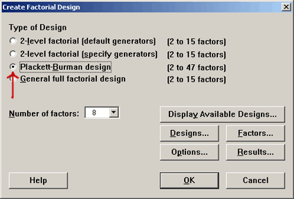
You specify how many runs and how many factors are in your experiment. If we specified eight factors and 12 runs, we get a design that looks like this:
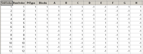
This look very much like the designs we had before. In this case we have eight factors, A through H, each with two levels. And each factor is defined by a 12 run design, 6 pluses and 6 minuses. Again, these are contrasts. Half of the observations at a high level and half at the low-level, and if you take any two columns they are orthogonal to each other. So, these are an orthogonal set of columns just as we had for the \(2^{k-p}\) design. If you take the product of any two of these and add them up, the sum of the products you get is zero.
Because these are orthogonal contrasts we get clean information on all main effects. The main effects are not confounded as required by the orthogonality of those columns.
Here is a quick way to manually create this type of design. First of all, one would fill out the first column of the design table, this would be column A. Then you can create the B column by taking the last element for permuting and then slide everything down. This process can be repeated for each column of factors needed in the design. Watch the video below to see how this works:
You can generate these designs by just knowing the first 11 elements, permuting these into the next column and adding an additional row of minuses across the bottom. It has this cyclical pattern and it works for most of these types of designs, (12, 20, 24, 36, but not for 28!). Here is what it looks like for 20 runs with 16 factors:
Placket - Burman Design
| Factors: | 16 | Replicates: | 1 |
| Base runs: | 20 | Total runs: | 20 |
| Base blocks: | 1 | Total blocks: | 1 |
Design Table
| Run | Blk | A | B | C | D | E | F | G | H | J | K | L | M | N | O | P | Q |
|---|---|---|---|---|---|---|---|---|---|---|---|---|---|---|---|---|---|
| 1 | 1 | + | - | + | + | - | - | - | - | + | - | + | - | + | + | + | + |
| 2 | 1 | + | + | - | + | + | - | - | - | - | + | - | + | - | + | + | + |
| 3 | 1 | - | + | + | - | + | + | - | - | - | - | + | - | + | - | + | + |
| 4 | 1 | - | - | + | + | - | + | + | - | - | - | - | + | - | + | - | + |
| 5 | 1 | + | - | - | + | + | - | + | + | - | - | - | - | + | - | + | - |
| 6 | 1 | + | + | - | - | + | + | - | + | + | - | - | - | - | + | - | + |
| 7 | 1 | + | + | + | - | - | + | + | - | + | + | - | - | - | - | + | - |
| 8 | 1 | + | + | + | + | - | - | + | + | - | + | + | - | - | - | - | + |
| 9 | 1 | - | + | + | + | + | - | - | + | + | - | + | + | - | - | - | - |
| 10 | 1 | + | - | + | + | + | + | - | - | + | + | - | + | + | - | - | - |
| 11 | 1 | - | + | - | + | + | + | + | - | - | + | + | - | + | + | - | - |
| 12 | 1 | + | - | + | - | + | + | + | + | - | - | + | + | - | + | + | - |
| 13 | 1 | - | + | - | + | - | + | + | + | + | - | - | + | + | - | + | + |
| 14 | 1 | - | - | + | - | + | - | + | + | + | + | - | - | + | + | - | + |
| 15 | 1 | - | - | - | + | - | + | - | + | + | + | + | - | - | + | + | - |
| 16 | 1 | - | - | - | - | + | - | + | - | + | + | + | + | - | - | + | + |
| 17 | 1 | + | - | - | - | - | + | - | + | - | + | + | + | + | - | - | + |
| 18 | 1 | + | + | - | - | - | - | + | - | + | - | + | + | + | + | - | - |
| 19 | 1 | - | + | + | - | - | - | - | + | - | + | - | + | + | + | + | - |
| 20 | 1 | - | - | - | - | - | - | - | - | - | - | - | - | - | - | - | - |
The cyclical pattern is a result of number theory properties that generate these orthogonal arrays. There is a lot of mathematical research behind these designs to achieve a matrix with orthogonal columns which is what we need.
We point out that these designs are a little different than the \(2^{k-p}\) designs. When you have a \(2^{k-p}\) design you have an alias structure that confounds some factors with other factors. Let's look at two examples to illustrate this.
Example: Fractional Factorial Design
Download: FF2LevelCorr.mpx
The first is a fractional factorial, 4 factor design, Resolution IV with one generator ABCD or D = ABC. From this design, we get an alias structure that we are familiar with. Main effects are aliased with 3-way interactions which means that they are completely confounded with those factors. Two-way interactions are confounded with each other.
Fractional Factorial Design
| Factors: | 4 | Base Design: | 4, 8 | Resolution: | IV |
| Runs: | 8 | Replicates: | 1 | Fraction: | 1/2 |
| Blocks: | 1 | Center pts (total): | 0 | ||
Design Generators: D = ABC
Alias Structure
I + ABCD
A + BCD
B + ACD
C + ABD
D + ABC
AB + CD
AC + BD
AD + BC
Let's look at the correlation among these factors, A, B, C and D, and then a couple of interaction columns.
Correlations: A, B, C, D, AB, ABC, CD
| A | B | C | D | AB | ABC | |
|---|---|---|---|---|---|---|
| B | 0.000 1.000 |
|||||
| C | 0.000 1.000 |
0.000 1.000 |
||||
| D | 0.000 1.000 |
0.000 1.000 |
0.000 1.000 |
|||
| AB | 0.000 1.000 |
0.000 1.000 |
0.000 1.000 |
0.000 1.000 |
||
| ABC | 0.000 1.000 |
0.000 1.000 |
0.000 1.000 |
1.000 * |
0.000 1.000 |
|
| CD | 0.000 1.000 |
0.000 1.000 |
0.000 1.000 |
0.000 1.000 |
1.000 * |
0.000 1.000 |
This is just a simple Pearson correlation. What Minitab gives us is the coefficient and the p-value. We can ignore the p-values because we are not really interested in testing, however a correlation between A and B = 0, A and C = 0, A and D = 0, etc. The correlation between all these factors = 0 because of the orthogonality.
Look back up at the alias structure and you will see the D is confounded with ABC. As we look back at the correlation table the correlation between D and ABC = 1. The correlation between two factors that are confounded = 1. This is appropriate because they are completely correlated with each other. Therefore, in these \(2^{k-p}\) designs we can see through correlation that factors are either orthogonal (correlation = 0) or they are completely confounded (correlation = 1).
Next, let's look at the Plackett-Burman designs and see how this differs. Below, we have created a design for 9 factors, 12 runs and we are looking at the correlation among the main effects, A, B, C, D, and E.
Plackett - Burman Design
| Factors: | 9 | Replicates: | 1 |
| Base runs: | 12 | Total runs: | 12 |
| Base blocks: | 1 | Total blocks: | 1 |
Correlations: A, B, C, D, E
| A | B | C | D | |
|---|---|---|---|---|
| B | 0.000 1.000 |
|||
| C | 0.000 1.000 |
0.000 1.000 |
||
| D | 0.000 1.000 |
0.000 1.000 |
0.000 1.000 |
|
| E | 0.000 1.000 |
0.000 1.000 |
0.000 1.000 |
0.000 1.000 |
These are the main factors themselves already set in orthogonal columns so these correlations = 0. If we look at the next design, however, in this case, we have the 12 runs and then we have created new 2-way interactions through multiplication of the factors already determined. Again, ignoring the p-values we produced a correlation matrix, (partially displayed below).
Correlations: AB, A, B, C, D, F, G, H, J, AB, AC, AD
| AB | A | B | C | D | F | G | H | J | ||
|---|---|---|---|---|---|---|---|---|---|---|
| A | 0.000 1.000 |
|||||||||
| B | 0.000 1.000 |
0.000 1.000 |
||||||||
| C | -0.333 0.290 |
0.000 1.000 |
0.000 1.000 |
|||||||
| D | 0.333 1.290 |
0.000 1.000 |
0.000 1.000 |
0.000 1.000 |
||||||
| F | -0.333 0.290 |
0.000 1.000 |
0.000 1.000 |
0.000 1.000 |
0.000 1.000 |
|||||
| G | -0.333 0.290 |
0.000 1.000 |
0.000 1.000 |
0.000 1.000 |
0.000 1.000 |
0.000 1.000 |
||||
| H | 0.333 0.290 |
0.000 1.000 |
0.000 1.000 |
0.000 1.000 |
0.000 1.000 |
0.000 1.000 |
0.000 1.000 |
|||
| J | -0.333 0.290 |
0.000 1.000 |
0.000 1.000 |
0.000 1.000 |
0.000 1.000 |
0.000 1.000 |
0.000 1.000 |
0.000 1.000 |
0.000 1.000 |
|
| AB | 1.000 * |
0.000 1.000 |
0.000 1.000 |
-0.333 0.290 |
0.333 0.290 |
-0.333 0.290 |
-0.333 0.290 |
0.333 0.290 |
-0.333 0.290 |
|
| AC | 0.000 1.000 |
0.000 1.000 |
-0.333 0.290 |
0.000 1.000 |
-0.333 0.290 |
0.333 0.290 |
-0.333 0.290 |
0.333 0.290 |
-0.333 0.290 |
|
| AD | 0.000 1.000 |
0.000 1.000 |
0.333 0.290 |
-0.333 0.290 |
0.000 1.000 |
-0.333 0.290 |
-0.333 0.290 |
-0.333 0.290 |
-0.333 0.290 |
A is orthogonal to every other factor, the correlation value = 0. B is not correlated with all the other main effects, where correlation = 0, but with some of these two-way interactions the correlation = 0.333. This shows partial confounding with the two-way interaction. Likewise, C has partial confounding with AB and AD. D is partially confounded with AB and AC. F is partially confounded with AB and AC and AD, ... and so forth.
Plackett-Burman designs have partial confounding, not complete confounding, with the 2-way and 3-way and higher interactions. Although they have this property that some effects are orthogonal they do not have the same structure allowing complete or orthogonal correlation with the other two way and higher order interactions.
Like other Resolution II designs, these designs are also good for screening for important factors. But remember, in a Resolution II design a main effect might look important because some combination of interactions is important and the main effect itself might not be the important effect.
If you assume that your interactions = 0 or are not important these are great designs. If your assumption is wrong and there are interactions, then it could show up as influencing one or the other main effects. These designs are very efficient with small numbers of observations and useful but remember the caveat, you are assuming that the main effects are going to show up as larger effects than interactions so that they will dominate the interaction effects.
Using Minitab we can ask for up to 47 factors. In doing so you want to select a sufficient number of runs over the number of factors so that you have a reasonable number of degrees of freedom for error. At this stage a statistical test really isn't that important, you are just screening for a place to start.
| [1] | Link |
| ↥ | Has Tooltip/Popover |
| Toggleable Visibility |