8.4 - Plackett-Burman Designs
8.4 - Plackett-Burman DesignsWe looked at \(2^{k-p}\) designs, which give us designs that have 8, 16, 32, 64, 128, etc. number of runs. We noted that all of these numbers are some fraction of \(1/2^{p}\) of a \(2^k\) design.
However, when you look at these numbers there is a pretty big gap between 16 and 32, 32 to 64, etc. We sometimes need other alternative designs besides these with a different number of observations.
A class of designs that allows us to create experiments with some number between these fractional factorial designs are the Plackett-Burman designs. Plackett-Burman designs exist for
N = 12, [16], 20, 24, 28, [32], 36, 40, 44, 48, ...
... any number which is divisible by four. These designs are similar to Resolution III designs, meaning you can estimate main effects clear of other main effects. Main effects are clear of each other but they are confounded with other higher interactions.
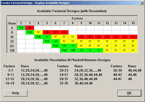
Look at the table of available designs in Minitab. The Plackett-Burman designs are listed below:

So, if you have 2 to 7 factors you can create a Plackett-Burman design with 12, 20, 24, ... up to 48 observations. Of course, if you have 7 factors with eight runs then you have a saturated design.
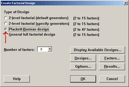
In the textbook there is a brief shortcut way of creating these designs, but in Minitab we simply select the Plackett-Burman option.

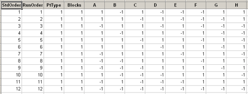
You specify how many runs and how many factors are in your experiment. If we specified eight factors and 12 runs, we get a design that looks like this:

This look very much like the designs we had before. In this case we have eight factors, A through H, each with two levels. And each factor is defined by a 12 run design, 6 pluses and 6 minuses. Again, these are contrasts. Half of the observations at a high level and half at the low-level, and if you take any two columns they are orthogonal to each other. So, these are an orthogonal set of columns just as we had for the \(2^{k-p}\) design. If you take the product of any two of these and add them up, the sum of the products you get is zero.
Because these are orthogonal contrasts we get clean information on all main effects. The main effects are not confounded as required by the orthogonality of those columns.
Here is a quick way to manually create this type of design. First of all, one would fill out the first column of the design table, this would be column A. Then you can create the B column by taking the last element for permuting and then slide everything down. This process can be repeated for each column of factors needed in the design. Watch the video below to see how this works:
You can generate these designs by just knowing the first 11 elements, permuting these into the next column and adding an additional row of minuses across the bottom. It has this cyclical pattern and it works for most of these types of designs, (12, 20, 24, 36, but not for 28!). Here is what it looks like for 20 runs with 16 factors:
Placket - Burman Design
| Factors: | 16 | Replicates: | 1 |
| Base runs: | 20 | Total runs: | 20 |
| Base blocks: | 1 | Total blocks: | 1 |
Design Table
| Run | Blk | A | B | C | D | E | F | G | H | J | K | L | M | N | O | P | Q |
|---|---|---|---|---|---|---|---|---|---|---|---|---|---|---|---|---|---|
| 1 | 1 | + | - | + | + | - | - | - | - | + | - | + | - | + | + | + | + |
| 2 | 1 | + | + | - | + | + | - | - | - | - | + | - | + | - | + | + | + |
| 3 | 1 | - | + | + | - | + | + | - | - | - | - | + | - | + | - | + | + |
| 4 | 1 | - | - | + | + | - | + | + | - | - | - | - | + | - | + | - | + |
| 5 | 1 | + | - | - | + | + | - | + | + | - | - | - | - | + | - | + | - |
| 6 | 1 | + | + | - | - | + | + | - | + | + | - | - | - | - | + | - | + |
| 7 | 1 | + | + | + | - | - | + | + | - | + | + | - | - | - | - | + | - |
| 8 | 1 | + | + | + | + | - | - | + | + | - | + | + | - | - | - | - | + |
| 9 | 1 | - | + | + | + | + | - | - | + | + | - | + | + | - | - | - | - |
| 10 | 1 | + | - | + | + | + | + | - | - | + | + | - | + | + | - | - | - |
| 11 | 1 | - | + | - | + | + | + | + | - | - | + | + | - | + | + | - | - |
| 12 | 1 | + | - | + | - | + | + | + | + | - | - | + | + | - | + | + | - |
| 13 | 1 | - | + | - | + | - | + | + | + | + | - | - | + | + | - | + | + |
| 14 | 1 | - | - | + | - | + | - | + | + | + | + | - | - | + | + | - | + |
| 15 | 1 | - | - | - | + | - | + | - | + | + | + | + | - | - | + | + | - |
| 16 | 1 | - | - | - | - | + | - | + | - | + | + | + | + | - | - | + | + |
| 17 | 1 | + | - | - | - | - | + | - | + | - | + | + | + | + | - | - | + |
| 18 | 1 | + | + | - | - | - | - | + | - | + | - | + | + | + | + | - | - |
| 19 | 1 | - | + | + | - | - | - | - | + | - | + | - | + | + | + | + | - |
| 20 | 1 | - | - | - | - | - | - | - | - | - | - | - | - | - | - | - | - |
The cyclical pattern is a result of number theory properties that generate these orthogonal arrays. There is a lot of mathematical research behind these designs to achieve a matrix with orthogonal columns which is what we need.
We point out that these designs are a little different than the \(2^{k-p}\) designs. When you have a \(2^{k-p}\) design you have an alias structure that confounds some factors with other factors. Let's look at two examples to illustrate this.
Example: Fractional Factorial Design
Download: FF2LevelCorr.mpx
The first is a fractional factorial, 4 factor design, Resolution IV with one generator ABCD or D = ABC. From this design, we get an alias structure that we are familiar with. Main effects are aliased with 3-way interactions which means that they are completely confounded with those factors. Two-way interactions are confounded with each other.
Fractional Factorial Design
| Factors: | 4 | Base Design: | 4, 8 | Resolution: | IV |
| Runs: | 8 | Replicates: | 1 | Fraction: | 1/2 |
| Blocks: | 1 | Center pts (total): | 0 | ||
Design Generators: D = ABC
Alias Structure
I + ABCD
A + BCD
B + ACD
C + ABD
D + ABC
AB + CD
AC + BD
AD + BC
Let's look at the correlation among these factors, A, B, C and D, and then a couple of interaction columns.
Correlations: A, B, C, D, AB, ABC, CD
| A | B | C | D | AB | ABC | |
|---|---|---|---|---|---|---|
| B | 0.000 1.000 |
|||||
| C | 0.000 1.000 |
0.000 1.000 |
||||
| D | 0.000 1.000 |
0.000 1.000 |
0.000 1.000 |
|||
| AB | 0.000 1.000 |
0.000 1.000 |
0.000 1.000 |
0.000 1.000 |
||
| ABC | 0.000 1.000 |
0.000 1.000 |
0.000 1.000 |
1.000 * |
0.000 1.000 |
|
| CD | 0.000 1.000 |
0.000 1.000 |
0.000 1.000 |
0.000 1.000 |
1.000 * |
0.000 1.000 |
This is just a simple Pearson correlation. What Minitab gives us is the coefficient and the p-value. We can ignore the p-values because we are not really interested in testing, however a correlation between A and B = 0, A and C = 0, A and D = 0, etc. The correlation between all these factors = 0 because of the orthogonality.
Look back up at the alias structure and you will see the D is confounded with ABC. As we look back at the correlation table the correlation between D and ABC = 1. The correlation between two factors that are confounded = 1. This is appropriate because they are completely correlated with each other. Therefore, in these \(2^{k-p}\) designs we can see through correlation that factors are either orthogonal (correlation = 0) or they are completely confounded (correlation = 1).
Next, let's look at the Plackett-Burman designs and see how this differs. Below, we have created a design for 9 factors, 12 runs and we are looking at the correlation among the main effects, A, B, C, D, and E.
Plackett - Burman Design
| Factors: | 9 | Replicates: | 1 |
| Base runs: | 12 | Total runs: | 12 |
| Base blocks: | 1 | Total blocks: | 1 |
Correlations: A, B, C, D, E
| A | B | C | D | |
|---|---|---|---|---|
| B | 0.000 1.000 |
|||
| C | 0.000 1.000 |
0.000 1.000 |
||
| D | 0.000 1.000 |
0.000 1.000 |
0.000 1.000 |
|
| E | 0.000 1.000 |
0.000 1.000 |
0.000 1.000 |
0.000 1.000 |
These are the main factors themselves already set in orthogonal columns so these correlations = 0. If we look at the next design, however, in this case, we have the 12 runs and then we have created new 2-way interactions through multiplication of the factors already determined. Again, ignoring the p-values we produced a correlation matrix, (partially displayed below).
Correlations: AB, A, B, C, D, F, G, H, J, AB, AC, AD
| AB | A | B | C | D | F | G | H | J | ||
|---|---|---|---|---|---|---|---|---|---|---|
| A | 0.000 1.000 |
|||||||||
| B | 0.000 1.000 |
0.000 1.000 |
||||||||
| C | -0.333 0.290 |
0.000 1.000 |
0.000 1.000 |
|||||||
| D | 0.333 1.290 |
0.000 1.000 |
0.000 1.000 |
0.000 1.000 |
||||||
| F | -0.333 0.290 |
0.000 1.000 |
0.000 1.000 |
0.000 1.000 |
0.000 1.000 |
|||||
| G | -0.333 0.290 |
0.000 1.000 |
0.000 1.000 |
0.000 1.000 |
0.000 1.000 |
0.000 1.000 |
||||
| H | 0.333 0.290 |
0.000 1.000 |
0.000 1.000 |
0.000 1.000 |
0.000 1.000 |
0.000 1.000 |
0.000 1.000 |
|||
| J | -0.333 0.290 |
0.000 1.000 |
0.000 1.000 |
0.000 1.000 |
0.000 1.000 |
0.000 1.000 |
0.000 1.000 |
0.000 1.000 |
0.000 1.000 |
|
| AB | 1.000 * |
0.000 1.000 |
0.000 1.000 |
-0.333 0.290 |
0.333 0.290 |
-0.333 0.290 |
-0.333 0.290 |
0.333 0.290 |
-0.333 0.290 |
|
| AC | 0.000 1.000 |
0.000 1.000 |
-0.333 0.290 |
0.000 1.000 |
-0.333 0.290 |
0.333 0.290 |
-0.333 0.290 |
0.333 0.290 |
-0.333 0.290 |
|
| AD | 0.000 1.000 |
0.000 1.000 |
0.333 0.290 |
-0.333 0.290 |
0.000 1.000 |
-0.333 0.290 |
-0.333 0.290 |
-0.333 0.290 |
-0.333 0.290 |
A is orthogonal to every other factor, the correlation value = 0. B is not correlated with all the other main effects, where correlation = 0, but with some of these two-way interactions the correlation = 0.333. This shows partial confounding with the two-way interaction. Likewise, C has partial confounding with AB and AD. D is partially confounded with AB and AC. F is partially confounded with AB and AC and AD, ... and so forth.
Plackett-Burman designs have partial confounding, not complete confounding, with the 2-way and 3-way and higher interactions. Although they have this property that some effects are orthogonal they do not have the same structure allowing complete or orthogonal correlation with the other two way and higher order interactions.
Like other Resolution II designs, these designs are also good for screening for important factors. But remember, in a Resolution II design a main effect might look important because some combination of interactions is important and the main effect itself might not be the important effect.
If you assume that your interactions = 0 or are not important these are great designs. If your assumption is wrong and there are interactions, then it could show up as influencing one or the other main effects. These designs are very efficient with small numbers of observations and useful but remember the caveat, you are assuming that the main effects are going to show up as larger effects than interactions so that they will dominate the interaction effects.
Using Minitab we can ask for up to 47 factors. In doing so you want to select a sufficient number of runs over the number of factors so that you have a reasonable number of degrees of freedom for error. At this stage a statistical test really isn't that important, you are just screening for a place to start.