11.2 - Response Surface Designs
11.2 - Response Surface DesignsAfter using the Steepest Ascent method to find the optimum location in terms of our factors, we can now go directly to the second order response surface design. A favorite design that we consider for a second order model is referred to as a central composite design.
Here is an example in two dimensions: Example 11.2 in the text. We have \(2^k\) corner points and we have some number of center points which generally would be somewhere between 4 and 7, (five here). In two dimensions there are 4 star points, but in general there are \(2^k\) star points in \(k\) dimensions. The value of these points is something greater than 1. Why is it something greater than 1? If you think about the region of experimentation, we have up to now always defined a box, but if you think of a circle the star points are somewhere on the circumference of that circle, or in three dimensions on the ball enclosing the box. All of these are design points around the region where you expect the optimum outcome to be located. Typically the only replication, in order to get some measure of pure error, is done at the center of the design.
The data set for the Example 11.2 is found in the Minitab worksheet, Ex11-2.mwx | Ex11-2.csv. The analysis using the Response Surface Design analysis module is shown in the Ex11-2.mpx.
11.2.1 - Central Composite Designs
11.2.1 - Central Composite DesignsIn the last section we looked at the Example 11.2 which was in coded variables and was a central composite design.
In this section we examine a more general central composite design. For \(k = 2\) we had a \(2^2\) design with center points, which was required for our first order model; then we added \(2*k\) star points. The star or axial points are, in general, at some value \(\alpha\) and \({-\alpha}\) on each axis.
There are various choices of α. If \(\alpha = 1\), the star points would be right on the boundary, and we would just have a \(3^2\) design. Thus \(\alpha = 1\) is a special case, a case that we considered in the \(3^k\) designs. A more common choice of \(\alpha\) is \(\alpha =\sqrt{k}\) which gives us a spherical design as shown below.
Our \(2^2\) design gives us the box, and adding the axial points (in green) outside of the box gives us a spherical design where \(\alpha =\sqrt{k}\). The corner points and the axial points at \(\alpha\), are all points on the surface of a ball in three dimensions, as we see below.
This design in \(k = 3\) dimensions can also be referred to as a central composite design, chosen so that the design is spherical. This is a common design. Much of this detail is given in Table 11.11 of the text.
An alternative choice where \(\alpha = \left ( n_{F} \right )^{\frac{1}{4}}\), or the fourth root of the number of points in the factorial part of the design, gives us a rotatable design.
If we have k factors, then we have, \(2^k\) factorial points, \(2*k\) axial points and \(n_{c}\) center points. Below is a table that summarizes these designs and compares them to \(3^k\) designs:
| k = 2 | k = 3 | k = 4 | k = 5 | ||
|---|---|---|---|---|---|
| Central Composite Designs | Factorial points \(\mathbf{2^k}\) | 4 | 8 | 16 | 32 |
| Star points \(\mathbf{2^k}\) | 4 | 6 | 8 | 10 | |
| Center points \(\mathbf{n_c}\) (varies) | 5 | 5 | 6 | 6 | |
| Total | 13 | 19 | 30 | 48 | |
| \(\mathbf{3^k}\) Designs | 9 | 27 | 81 | 243 | |
| Choice of \(\alpha\) | Spherical design ( \(\mathbf{\alpha =\sqrt{k}}\) ) | 1.4 | 1.73 | 2 | 2.24 |
| Rotatable design ( \(\mathbf{\alpha = \left ( n_{F} \right )^{\frac{1}{4}}}\) ) | 1.4 | 1.68 | 2 | 2.38 | |
Compare the total number of observations required in the central composite designs versus the \(3^k\) designs. As the number of factors increases, you can see the efficiencies that are brought to bear.
The spherical designs are rotatable in the sense that the points are all equidistant from the center. Rotatable refers to the variance of the response function. A rotatable design exists when there is an equal prediction variance for all points a fixed distance from the center, 0. This is a nice property. If you pick the center of your design space and run your experiments, all points that are equal distance from the center in any direction, have an equal variance of prediction.
You can see in the table above that the difference in the variation between the spherical and rotatable designs are slight, and don't seem to make much difference. But both ideas provide justification for selecting how far away the star points should be from the center.
Why do we take about five or six center points in the design? The reason is also related to the variance of a predicted value. When fitting a response surface you want to estimate the response function in this design region where we are trying to find the optimum. We want the prediction to be reliable throughout the region, and especially near the center since we hope the optimum is in the central region. By picking five to six center points, the variance in the middle is approximately the same as the variance at the edge. If you only had one or two center points, then you would have less precision in the middle than you would have at the edge. As you go farther out beyond a distance of 1 in coded units, you get more variance and less precision. What we are trying to do is to balance the precision at the edge of the design relative to the middle.
How do you select the region where you want to run the experiment? Remember, for each factor X we said we need to choose the lower level is and the upper level for the region of experimentation. We usually picked the -1 and 1 as the boundary. If the lower natural unit is really the lowest number that you can test, because the experiment won't work lower than this, or the lower level is zero and you can't put in a negative amount of something, then, the star point is not possible because it is outside the range of experimentation.
If this is the case, one choice that you could make would be to use the \({-\alpha}\) as the lowest point. Generally, if you are not up against a boundary then this is not an issue and the star points are a way to reach beyond the region that you think the experiment should be run in. The issue isn't selecting the coding of the design relative to the natural units. You might lose some of these exact properties, but as long as you have the points nicely spread out in space you can fit a regression function. The penalty for not specifying the points exactly would be seen in the variance, and it would be actually very slight.
Minitab® – Generating These Designs in Minitab
Minitab will show you the available designs and how to generate these designs.

We can create central composite designs using a full factorial, central composite designs with fractional factorials, half fraction and a quarter fraction, and they can be arranged in blocks. Later, we will look at the Box-Behnken designs.
As an example, we look at the \(k=3\) design, set up in Minitab using a full factorial, completely randomized, in two blocks, or three blocks with six center points and the default \(\alpha = 1.633\) (or \(\alpha = 1.682\) for a rotatable design).
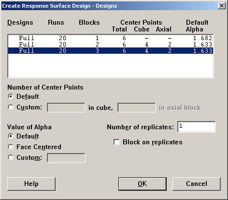
If you do not want the default \(\alpha\) you can specify your own in the lower left. A Face Centered design is obtained by putting the \(\alpha\) at +1 and -1 on the cube. Here is the design that results:
| Run | Blk | A | B | C |
|---|---|---|---|---|
| 1 | 1 | -1.000 | -1.000 | -1.000 |
| 2 | 1 | 1.000 | 1.000 | -1.000 |
| 3 | 1 | 1.000 | -1.000 | 1.000 |
| 4 | 1 | -1.000 | 1.000 | 1.000 |
| 5 | 1 | 0.000 | 0.000 | 0.000 |
| 6 | 1 | 0.000 | 0.000 | 0.000 |
| 7 | 2 | 1.000 | -1.000 | -1.000 |
| 8 | 2 | -1.000 | 1.000 | -1.000 |
| 9 | 2 | -1.000 | -1.000 | 1.000 |
| 10 | 2 | 1.000 | 1.000 | 1.000 |
| 11 | 2 | 0.000 | 0.000 | 0.000 |
| 12 | 2 | 0.000 | 0.000 | 0.000 |
| 13 | 3 | -1.633 | 0.000 | 0.000 |
| 14 | 3 | 1.633 | 0.000 | 0.000 |
| 15 | 3 | 0.000 | -1.633 | 0.000 |
| 16 | 3 | 0.000 | 1.633 | 0.000 |
| 17 | 3 | 0.000 | 0.000 | -1.633 |
| 18 | 3 | 0.000 | 0.000 | 1.633 |
| 19 | 3 | 0.000 | 0.000 | 0.000 |
| 20 | 3 | 0.000 | 0.000 | 0.000 |
The first block is a one half fraction of the \(2^3\) plus two center points. Block 2 is the second half fraction of the factorial part with two center points. The third block consists of six star points, plus to center points. Each of the three blocks contains two center points and the first two blocks have half of the corner points each. The third block contains the star points and is of size 8.
Rollover the words 'Block 1', 'Block 2', and 'Block 3' in the graphic above. Do you see how they use center points strategically to tie the blocks together? They are represented in each block and they keep the design connected.
The corner points all have +1 or -1 for every dimension, because they're at the corners. They are either up or down, in or out, right or left. The axial points have \(+\alpha\), or \(-\alpha\) \((+1.6330\ or -1.6330)\) for A, but are 0 for factors B and C. The center points have zero on all three axes, truly the center of this region. We have designed this to cover the space in just the right way so that we can estimate a quadratic equation. Using a Central Composite Design, we can't estimate cubic terms, and we can't estimate higher order interactions. If we had utilized a \(3^k\) design, one that quickly becomes unreasonably large, then we would have been able to estimate all of the higher order interactions.
However, we would have wasted a lot of resources to do it. The CCD allows us to estimate just linear and quadratic terms and first order interactions.
Example 11.1: Polymers and Elasticity
This example is from the Box and Draper (1987) book and the data from Tables 9.2 and 9.4 are in Minitab (BD9-1.csv).
This example has three variables and they are creating a polymer, a kind of plastic that has a quality of elasticity. The measurement in this experiment is the level of elasticity. We created the design in Minitab for this experiment, however the data only has two center points:
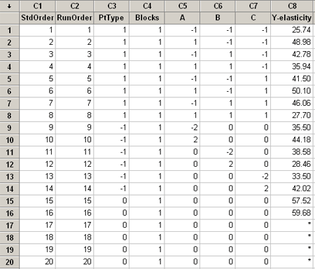
Variables A and B are the concentration of two ingredients that make up the polymer, and C is the temperature, and the response is elasticity. There are 8 corner points, a complete factorial, 6 star points and 2 center points.
Let's go right to the analysis stage now using Minitab ...
or you can view the condensed version with no audio...
Before we move on I would like to go back and take a look again at the plot of the residuals. Wait a minute! Is there something wrong with this residual plot?
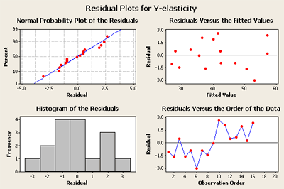
Residual plot for the polynomial fit
Look at the plot in the lower right. The first eight points tend to be low, and then the next eight points are at a higher level. This is a clue, that something is influencing the response that is not being fit by the model. This looks suspicious. What happened? My guess is that the experiment was run in two phases. They first ran the \(2^k\) part - (block 1). And then they noticed the response and added the star points to make a responsive surface design in the second part. This is often how these experiments are conducted. You first perform a first-order experiment, and then you add center points and star points and then fit the quadratic.
Add a block term and rerun the experiment to see if this makes a difference.
Two Types of Central Composite Designs
The central composite design has \(2*k\) star points on the axial lines outside of the box defined by the corner points. There are two major types of central composite designs: the spherical central composite design where the star points are the same distance from the center as the corner points, and the rotatable central composite design where the star points are shifted or placed such that the variances of the predicted values of the responses are all equal, for x’s which are an equal distance from the center.
When you are choosing, in the natural units, the values corresponding to the low and high, i.e. corresponding to -1 and 1 in coded units, keep in mind that the design will have to include points further from the center in all directions. You are trying to fit the design in the middle of your region of interest, the region where you expect the experiment to give the optimal response.
11.2.2 - Box-Behnken Designs
11.2.2 - Box-Behnken DesignsBox-Behnken Designs
Another class of response surface designs are called Box-Behnken designs. They are very useful in the same setting as the central composite designs. Their primary advantage is in addressing the issue of where the experimental boundaries should be, and in particular to avoid treatment combinations that are extreme. By extreme, we are thinking of the corner points and the star points, which are extreme points in terms of region in which we are doing our experiment. The Box-Behnken design avoids all the corner points, and the star points.
One way to think about this is that in the central composite design we have a ball where all of the corner points lie on the surface of the ball. In the Box-Behnken design the ball is now located inside the box defined by a 'wire frame' that is composed of the edges of the box. If you blew up a balloon inside this wire frame box so that it just barely extends beyond the sides of the box, it might look like this, in three dimensions. Notice where the balloon first touches the wire frame; this is where the points are selected to create the design.
Box-Behnken Design
| Factors: | 3 | Replicates: | 1 |
| Base runs: | 15 | Total runs: | 15 |
| Base Blocks: | 1 | Total Blocks: | 1 |
| Center points: | 3 | ||
Design Table
| Run | Blk | A | B | C |
|---|---|---|---|---|
| 1 | 1 | - | - | 0 |
| 2 | 1 | + | - | 0 |
| 3 | 1 | - | + | 0 |
| 4 | 1 | + | + | 0 |
| 5 | 1 | - | 0 | - |
| 6 | 1 | + | 0 | - |
| 7 | 1 | - | 0 | + |
| 8 | 1 | + | 0 | + |
| 9 | 1 | 0 | - | - |
| 10 | 1 | 0 | + | - |
| 11 | 1 | 0 | - | + |
| 12 | 1 | 0 | + | + |
| 13 | 1 | 0 | 0 | 0 |
| 14 | 1 | 0 | 0 | 0 |
| 15 | 1 | 0 | 0 | 0 |
Therefore the points are still on the surface of a ball, but the points are never further out than the low and high in any direction. In addition, there would be multiple center points as before. In this type of design, you do not need as many center points because points on the outside are closer to the middle. The number of center points are again chosen so that the variance of is about the same in the middle of the design as it is on the outside of the design.
In Minitab, we can see the different designs that are available. Listed at the bottom are the Box-Behnken Designs.
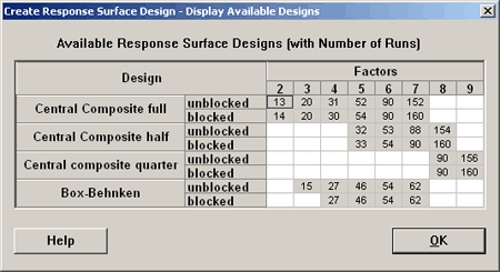
A Box-Behnken (BB) design with two factors does not exist. With three factors the BB design by default will have three center points and is given in the Minitab output shown above. The last three observations are the center points. The other points, you will notice, all include one 0 for one of the factors and then a plus or minus combination for the other two factors.
If you consider the BB design with four factors, you get the same pattern where we have two of the factors at + or - 1 and the other two factors are 0. Again, this design has three center points and a total of 27 observations.
Comparing the central composite design with 4 factors, which has 31 observations, a Box-Behnken design only includes 27 observations. For 5 factors, the Box-Behnken would have 46 observations, and a central composite would have 52 observations if you used a complete factorial, but this is where the central composite also allows you to use a fractional factorial as a means of making this experiment more efficient. Likewise, for six factors, the Box-Behnken requires 54 observations, and this is the minimum of the central composite design.
Both the CCD and the BB design can work, but they have different structures, so if your experimental region is such that extreme points are a problem then there are some advantages to the Box-Behnken. Otherwise, they both work well.
The central composite design is one that I favor because even though you are interested in the middle of a region if you put all your points in the middle you do not have as much leverage about where the model fits. So when you can move your points out you get better information about the function within your region of experimentation.
However, by moving your points too far out, you get into boundaries or could get into extreme conditions, and then enter the practical issues which might outweigh the statistical issues. The central composite design is used more often but the Box-Behnken is a good design in the sense that you can fit the quadratic model. It would be interesting to look at the variance of the predicted values for both of these designs. (This would be an interesting research question for somebody!) The question would be which of the two designs gives you a smaller average variance over the region of experimentation.
The usual justification for going to the Box-Behnken is to avoid the situation where the corner points in the central composite design are very extreme, i.e. they are at the highest level of several factors. So, because they are very extreme, the researchers may say these points are not very typical. In this case, the Box Behnken may look a lot more desirable since there are more points in the middle of the range and they are not as extreme. The Box-Behnken might feel a little 'safer' since the points are not as extreme as all of the factors.
The Variance of the Predicted Values
Let's look at this a little bit. We can write out the model:
\(\hat{y}_{x} = b_0 + b_{1}x_{1} + b_{2}x_{2} + b_{11}x_{1}^{2} + b_{22}x_{2}^{2} + b_{12}x_{1}x_{2}\)
Where the b0, b1, etc are the estimated parameters. This is a quadratic model with two x's. The question we want to answer is how many center points should there be so that the variance of the predicted value, var(\(\hat{y}_{x}\)) when x is at the center is the same as when x is at the outside of the region?
See handout Chapter 11: Supplemental Text Material. This shows the impact on the variance of predicted value in the situation with k = 2, full factorial and the design has only 2 center points rather than the 5 or 6 that the central composite design would recommend.
What you see (S11-3) is that in the middle of the region the variance is much higher than further out. So, by putting more points in the center of the design, collecting more information there, (replicating a design in the middle), you see that the standard error is lower in the middle and roughly the same as farther out. It gets larger again in the corners and continues growing as you go out from the center. By putting in enough center points you balance the variance in the middle of the region relative to further out.
Another example (S11-4) is a central composite design where the star points are on the face. It is not rotatable design and the variance changes depending on which direction you're moving out from center of the design.
It also shows another example (S11-4), also a face-centered design with zero center points, which shows a slight hump in the middle on the variance function.
Notice that we only need two center points for the face-centered design. Rather than having our star points farther out, if we move them closer into the face we do not need as many center points because we already have points closer to the center. A lot of factors affect the efficiencies of these designs.
Rotatability
Rotatability is determined by our choice of alpha. A design is rotatable if the prediction variance depends only on the distance of the design point from the center of the design. This is what we were observing previously. Here in the supplemental material (S11-5) is an example with a rotatable design, but the variance contours are based on a reduced model. It only has one quadratic term rather than two. As a result we get a slightly different shape, the point being that rotatability and equal variance contours depend both on the design and on the model that we are fitting. We are usually thinking about the full quadratic model when we make that claim.