11.3 - Mixture Experiments
11.3 - Mixture ExperimentsExample 11-2
This is another class of response surface designs where the components are not just levels of factors but a special set where the \(x_1, x_2, \dots\) are coded and are the components of the mixture such that the sum of the \(x_i = 1\). So, these make up the proportions of the mixture.
Examples
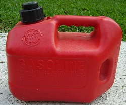
If you are making any kind of product it usually involves mixtures of ingredients. A classic example is gasoline which is a mixture of various petrochemicals. In polymer production, polymers are actually mixtures of components as well. My favorite classroom example is baking a cake. A cake is a mixture of flour, sugar, eggs, and other ingredients depending on the type of cake. It is a mixture where the levels of x are the proportions of the ingredients.
This constraint that the sum of the x's sum to 1, i.e.,
\(0 ≤ x_i ≤ 1\)
has an impact on how we analyze these experiments.
Here we will write out our usual linear model:
\(Y_i=\beta_0 + \beta_1x_{i1}+\beta_2x_{i2}+\ldots +\beta_kx_{ik}+\varepsilon_i\)
where, \(1 =\sum\limits_{j=1}^k x_{ij}\)
If you want to incorporate this constraint then we can write:
\(Y_i= \beta_1x_{i1}+\beta_2x_{i2}+\ldots +\beta_kx_{ik}+\varepsilon_i\)
in other words, if we drop the \(\beta_0\), this reduces the parameter space by 1 and then we can fit a reduced model even though the x's are each constrained.
In the quadratic model:
\(Y_h=\sum\limits_{i=1}^k \beta_i x_{hi}+\mathop{\sum\sum}\limits_{i<j}\beta_{ij}x_{hi}x_{hj}+\varepsilon_h\)
This is probably the model we are most interested in and will use the most. Then we can generalize this into a cubic model which has one additional term.
A Cubic Model
\(Y_h=\sum\limits_{i=1}^k \beta_i x_{hi} +\mathop{\sum\sum}\limits_{i<j}\beta_{ij}x_{hi}x_{hj}
+\mathop{\sum\limits^k\sum\limits^k\sum\limits^k}\limits_{i<j<l}\beta_{ijl}x_{hi}x_{hj}x_{hl}
+\varepsilon_h\)
These models are used to fit response surfaces.
Let's look at the parameter of space. Let's say that k = 2. The mixture is entirely made up of two ingredients, \(x_1\) and \(x_2\). The sum of both ingredients is a line plotted in the parameter space below: An experiment made up of two components is either all of \(x_1\) or all of \(x_2\) or something in between, a proportion of the two.
Let's take a Look at the parameter space in three dimensions. Here we have three components: \(x_1, x_2 \text{ and } x_3\). As we satisfy our constraint that the sum of all the components equal 1 and then our parameter space is the plane that cuts the three-dimensional surface, intersecting these three points in the graph below scratch that in the plot below.
Plot showing the plane where the sum: x1+x2+x3 = 1
The triangle represents the full extent of the region of experimentation in this case with the points sometimes referred to as the Barycentric coordinates. The design question we want to address is where do we do our experiment? We are not interested in any one of the corners of the triangle where only one ingredient is represented, we are interested in some way on the middle where there is a proportion of all three of the ingredients included. We will restrict it to a feasible region of experimentation somewhere in the middle area.
Let's look at an example, for instance, producing cattle feed. The ingredients might include the following: corn, oats, hay, soybean, grass, ... all sorts of things.
In some situations it might work where you might have 100% of one component, but many instances of mixtures we try to partition off a part of the space in the middle where we think the combination is optimal.
In k = 4 the region of experimentation can be represented by the shape of a tetrahedron where each of the four sides of the tetrahedron is an equalateral triangle and has its own set of Barycentric coordinates. Each face of the tetrahedron corresponds to design region where one coordinate is zero, and the remaining three must sum to 1.
11.3.1 - Two Major Types of Mixture Designs
11.3.1 - Two Major Types of Mixture DesignsSimplex Lattice Design
A {p,m} simplex lattice design for p factors (components) is defined as all possible combination of factor levels defined as
\(x_i=0,\frac{1}{m},\frac{2}{m},\cdots,1 \qquad i=1,2,\ldots,p\)
As an example, the simplex lattice design factor levels for the case of {3,2} will be
\(x_i=0,\frac{1}{2},1 \qquad i=1,2,3\)
Which results in the following design points:
\((x_1,x_2,x_3)=\{(1,0,0),(0,1,0),(0,0,1),(\frac{1}{2},\frac{1}{2},0),(\frac{1}{2},0,\frac{1}{2}),(0,\frac{1}{2},\frac{1}{2})\}\)
Simplex Centroid Design
This design which has \(2^{p}-1\) design points consist of p permutations of (1,0,0,…,0), permutations of \((1,0,0,\ldots,0),\displaystyle{p\choose 2}\), permutations of \((\dfrac{1}{2},\dfrac{1}{2},0,\ldots,0),\displaystyle{p\choose 3}\), and the overall centroid \(\displaystyle(\dfrac{1}{p},\dfrac{1}{p},\cdots,\dfrac{1}{p})\). Some simplex centroid designs for the case of p = 3 and p = 4 can be find in Figure 11.41.
Minitab handles mixture experiments which can be accessed through Stat > DOE > Mixture. It allows for building and analysis of Simplex Lattice and Simplex Centroid designs. Furthermore, it covers a third design which is named, Extreme Vertex Design. Application of Extreme Vertex designs are for cases where we have upper and lower constraints on some or all of the components making the design space smaller than the original region.
11.3.2 - Mixture Designs in Minitab
11.3.2 - Mixture Designs in MinitabHow does Minitab handle these types of experiments?
Mixture designs are a special case of response surface designs. Under the stat menu in many tab, select design of experiments, then mixture, create mixture design. Minitab then presents you with the following dialog box:
Simplex lattice option will look at the points that are extremes. Simplex lattice creates a design for p components of degree m. In this case, we want points that are made up of 0, \(1/m, 2/m, \dots\) up to 1. Classifying the points in this way tells us how we will space the points. For instance, if m = 2, then the only points we would have would be 0, 1/2, and 1 to play with in all key dimensions. You can create this design in Minitab, for 3 factors, using tab Stat > DOE > Mixture > Create Mixture Design and select Simplex Centroid. See the image here:
If we are in a design with the m = 3, then we would have 0, 1/3, 2/3, and 1. In this case we would have points a third of the way along each dimension. Any point on the boundary can be constructed in this way.
All of these points are on the boundary which means that they are made up of mixtures that omit one of the components. (This is not always desirable but in some settings it is fine.)
The centroid is the point in the middle. Axial points are points that lie along the lines that intersect the region of experimentation, points that are located interior and therefore include part of all of the components.
You can create this design in Minitab, for 3 factors, using tab Stat > DOE > Mixture > Create Mixture Design and select Simplex Centroid. See the image here:
This should give you the range of points that you think of when designing in a mixture. again, you want points in the middle but like regression in an unconstrained space you typically want to have your points farther out so you have good leverage. From this perspective, the points on the outside make a lot of sense. From an actual experimentation situation, you would have to be in a scientific setting also where those points make sense. If not, we would constrain this region to begin with. We will get in to this later.
How Rich of a Design?
Let's look at the set of possible designs that Minitab gives us.
Where it is labeled on the left Lattice 1, Lattice 2, etc., here minitab is referring to degree 1, 2, etc. So, if you want a lattice of degree 1, this is not very interesting. This means that you just have a 0 and 1. If you go to a lattice of degree 2 then you need six points in three dimensions. This is pretty much what we looked at previously... (roll over the red mixture points, below).
| Run | Type | A | B | C |
|---|---|---|---|---|
| 1 | 1 | 1.0000 | 0.0000 | 0.0000 |
| 2 | 2 | 0.5000 | 0.5000 | 0.0000 |
| 3 | 2 | 0.5000 | 0.0000 | 0.5000 |
| 4 | 1 | 0.0000 | 1.0000 | 0.0000 |
| 5 | 2 | 0.0000 | 0.5000 | 0.5000 |
| 6 | 1 | 0.0000 | 0.0000 | 1.0000 |
Here is a design table for a lattice with degree 3:
| Run | Type | A | B | C |
|---|---|---|---|---|
| 1 | 1 | 1.0000 | 0.0000 | 0.0000 |
| 2 | 2 | 0.6667 | 0.3333 | 0.0000 |
| 3 | 2 | 0.6667 | 0.0000 | 0.3333 |
| 4 | 2 | 0.3333 | 0.6667 | 0.0000 |
| 5 | 0 | 0.3333 | 0.3333 | 0.3333 |
| 6 | 2 | 0.3333 | 0.0000 | 0.6667 |
| 7 | 1 | 0.0000 | 1.0000 | 0.0000 |
| 8 | 2 | 0.0000 | 0.6667 | 0.3333 |
| 9 | 2 | 0.0000 | 0.3333 | 0.6667 |
| 10 | 1 | 0.0000 | 0.0000 | 1.0000 |
Now let's go into Minitab and augment this design by including axial points. Here is what results:
| Run | Type | A | B | C |
|---|---|---|---|---|
| 1 | 1 | 1.0000 | 0.0000 | 0.0000 |
| 2 | 2 | 0.6667 | 0.3333 | 0.0000 |
| 3 | 2 | 0.6667 | 0.0000 | 0.3333 |
| 4 | 2 | 0.3333 | 0.6667 | 0.0000 |
| 5 | 0 | 0.3333 | 0.3333 | 0.3333 |
| 6 | 2 | 0.3333 | 0.0000 | 0.6667 |
| 7 | 1 | 0.0000 | 1.0000 | 0.0000 |
| 8 | 2 | 0.0000 | 0.6667 | 0.3333 |
| 9 | 2 | 0.0000 | 0.3333 | 0.6667 |
| 10 | 1 | 0.0000 | 0.0000 | 1.0000 |
| 11 | -1 | 0.6667 | 0.1667 | 0.6667 |
| 12 | -1 | 0.1667 | 0.6667 | 0.1667 |
| 13 | -1 | 0.1667 | 0.1667 | 0.6667 |
This gives us three more points. Each of these points is 2/3, 1/6, 1/6. These are interior points.
These are good designs if you can run your experiment in the whole region.
Let's take a look at four dimensions and see what the program will do here. Here is a design with four components, four dimensions, and a lattice of degree three. We have also selected to augment this design with axial and center points.
| Run | Type | A | B | C | D |
|---|---|---|---|---|---|
| 1 | 1 | 1.0000 | 0.0000 | 0.0000 | 0.0000 |
| 2 | 2 | 0.6667 | 0.3333 | 0.0000 | 0.0000 |
| 3 | 2 | 0.6667 | 0.0000 | 0.3333 | 0.0000 |
| 4 | 2 | 0.6667 | 0.0000 | 0.0000 | 0.3333 |
| 5 | 2 | 0.3333 | 0.6667 | 0.0000 | 0.0000 |
| 6 | 3 | 0.3333 | 0.3333 | 0.3333 | 0.0000 |
| 7 | 3 | 0.3333 | 0.3333 | 0.0000 | 0.3333 |
| 8 | 2 | 0.3333 | 0.0000 | 0.6667 | 0.0000 |
| 9 | 3 | 0.3333 | 0.0000 | 0.3333 | 0.3333 |
| 10 | 2 | 0.3333 | 0.0000 | 0.0000 | 0.6667 |
| 11 | 1 | 0.0000 | 1.0000 | 0.0000 | 0.0000 |
| 12 | 2 | 0.0000 | 0.6667 | 0.3333 | 0.0000 |
| 13 | 2 | 0.0000 | 0.6667 | 0.0000 | 0.3333 |
| 14 | 2 | 0.0000 | 0.3333 | 0.6667 | 0.0000 |
| 15 | 3 | 0.0000 | 0.3333 | 0.3333 | 0.3333 |
| 16 | 2 | 0.0000 | 0.3333 | 0.0000 | 0.6667 |
| 17 | 1 | 0.0000 | 0.0000 | 1.0000 | 0.0000 |
| 18 | 2 | 0.0000 | 0.0000 | 0.6667 | 0.3333 |
| 19 | 2 | 0.0000 | 0.0000 | 0.3333 | 0.6667 |
| 20 | 1 | 0.0000 | 0.0000 | 0.0000 | 1.0000 |
| 21 | 0 | 0.2500 | 0.2500 | 0.2500 | 0.2500 |
| 22 | -1 | 0.6250 | 0.1250 | 0.1250 | 0.1250 |
| 23 | -1 | 0.1250 | 0.6250 | 0.1250 | 0.1250 |
| 24 | -1 | 0.1250 | 0.1250 | 0.6250 | 0.1250 |
| 25 | -1 | 0.1250 | 0.1250 | 0.1250 | 0.6250 |
This gives us 25 points in the design and the plot shows us the four faces of the tetrahedron. It doesn't look like it is showing us a plot of the interior points.
11.3.3 - The Analysis of Mixture Designs
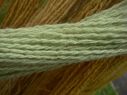
11.3.3 - The Analysis of Mixture DesignsExample 11.3: Elongation of Yarn
Download: Ex11-3.mwx | Ex11-3.csv
This example has to do with the elongation of yarn based on its component fabrics. There are three components in this mixture and each component is a synthetic material. The mixture design was one that we had looked at previously. It is a simple lattice design of degree 2. This means that it has mixtures of 0, 1/2, 100%. The components of this design are made up of these three possibilities.
| StdOrder | RunOrder | PtType | Blocks | A | B | C | Y | |
|---|---|---|---|---|---|---|---|---|
| 1 | 1 | 1 | 1 | 1 | 1.0 | 0.0 | 0.0 | 11.0 |
| 2 | 2 | 2 | 2 | 1 | 0.5 | 0.5 | 0.0 | 15.0 |
| 3 | 3 | 3 | 2 | 1 | 0.5 | 0.0 | 0.5 | 17.7 |
| 4 | 4 | 4 | 1 | 1 | 0.0 | 1.0 | 0.0 | 8.8 |
| 5 | 5 | 5 | 2 | 1 | 0.0 | 0.5 | 0.5 | 10.0 |
| 6 | 6 | 6 | 1 | 1 | 0.0 | 0.0 | 1.0 | 16.8 |
| 7 | 7 | 7 | 1 | 1 | 1.0 | 0.0 | 0.0 | 12.4 |
| 8 | 8 | 8 | 2 | 1 | 0.5 | 0.5 | 0.0 | 14.8 |
| 9 | 9 | 9 | 2 | 1 | 0.5 | 0.0 | 0.5 | 16.4 |
| 10 | 10 | 10 | 1 | 1 | 0.0 | 1.0 | 0.0 | 10.0 |
| 11 | 11 | 11 | 2 | 1 | 0.0 | 0.5 | 0.5 | 9.7 |
| 12 | 12 | 12 | 1 | 1 | 0.0 | 0.0 | 1.0 | 16.0 |
| 13 | 13 | 13 | 1 | 1 | 1.0 | 0.0 | 0.0 | * |
| 14 | 14 | 14 | 2 | 1 | 0.5 | 0.5 | 0.0 | 16.1 |
| 15 | 15 | 15 | 2 | 1 | 0.5 | 0.0 | 0.5 | 16.6 |
| 16 | 16 | 16 | 1 | 1 | 0.0 | 1.0 | 0.0 | * |
| 17 | 17 | 17 | 2 | 1 | 0.0 | 0.5 | 0.5 | 11.8 |
| 18 | 18 | 18 | 1 | 1 | 0.0 | 0.0 | 1.0 | * |
In the Minitab program, the first 6 runs show you the pure components, and in addition, you have the 5 mixed components. All of this was replicated 3 times so that we have 15 runs. There were three that had missing data.
You can also specify in more detail which type of points that you want to include in the mixture design using the dialog boxes in Minitab if your experiment requires this.
Analysis
In the analysis we fit the quadratic model ( the linear + the interaction terms). Remember we only have 6 points in this design, the vertex, the half-lengths, so we are fitting a response surface to these 6 points. Let's take a look at the analysis:
Regression for Mixtures: Y versus A, B, C
Estimated Regression Coefficients for Y (component proportions)
| Term | Coef | SE Coef | T | P | VIF |
|---|---|---|---|---|---|
| A | 11.70 | 0.6037 | * | * | 1.750 |
| B | 9.400 | 0.6037 | * | * | 1.750 |
| C | 16.400 | 0.637 | * | * | 1.750 |
| A*B | 19.000 | 2.6082 | 7.28 | 0.000 | 1.750 |
| A*C | 11.400 | 2.6082 | 4.37 | 0.002 | 1.750 |
| B*C | -9.600 | 2.6082 | -3.68 | 0.005 | 1.750 |
| S = 0.853750 | PRESS = 18.295 | |
| R-Sq = 95.14% | R- Sq(pred) = 86.43% | R-Sq(adj) = 92.43% |
Analysis of variance for Y (component proportions)
| Source | DF | Seq SS | Adj SS | Adj MS | F | P |
|---|---|---|---|---|---|---|
| Regression | 5 | 128.296 | 128.2960 | 25.6592 | 35.20 | 0.000 |
| Linear | 2 | 57.629 | 50.9200 | 25.4600 | 34.93 | 0.000 |
| Quadratic | 3 | 70.667 | 70.669 | 23.5556 | 32.32 | 0.000 |
| Residual Error | 9 | 6.560 | 6.5600 | 0.7289 | ||
| Total | 14 | 134.856 |
Here we get 2 df linear, 3 df quaratic, these are the five regression parameters. If you look at the individual coefficients, six of them because they are is no intercept, three linear and three cross-product terms... The 9 df for error are from the triple replicates and the double replicates. This is pure error and there is no additional df for lack of fit in this full model.
If we look at the coutour service plot we get:
We have the optimum somewhere between a mixture of A and C, with B essentially not contributing very much at all. So, roughly 2/3rds C and 1/3 A is what we would like in our mixture. Let's look at the optimizer to find the optimum values.
It looks like A = about .3 and B = about .7, with B not contributing nothing to the mixture.
Unless I see the plot how can I use the analysis output? How else can I determine the appropriate levels?
Example 11.4: Gasoline Production
Pr11-31.MTW from text
This example focuses on the production of an efficient gasoline mixture. The response variable is miles per gallon (mpg) as a function of the 3 components in the mixture. The data set contains these 14 points - which has duplicates at the centroid, labeled (1/3, 1/3, 1/3), and the three vertices, labeled (1,0,0), (0,1,0), and (0,0,1).
| StdOrder | RunOrder | PtType | Blocks | A | B | C | Y-mpg | |
|---|---|---|---|---|---|---|---|---|
| 1 | 1 | 1 | 1 | 1 | 1.00000 | 0.00000 | 0.00000 | 24.5 |
| 2 | 2 | 2 | 2 | 1 | 0.50000 | 0.50000 | 0.00000 | 25.1 |
| 3 | 3 | 3 | 2 | 1 | 0.50000 | 0.00000 | 0.50000 | 24.3 |
| 4 | 4 | 4 | 1 | 1 | 0.00000 | 1.00000 | 0.00000 | 24.8 |
| 5 | 5 | 5 | 2 | 1 | 0.00000 | 0.50000 | 0.50000 | 23.5 |
| 6 | 6 | 6 | 1 | 1 | 0.00000 | 0.00000 | 1.00000 | 22.7 |
| 7 | 7 | 7 | 0 | 1 | 0.33333 | 0.33333 | 0.33333 | 24.8 |
| 8 | 8 | 8 | -1 | 1 | 0.66667 | 0.16667 | 0.16667 | 24.2 |
| 9 | 9 | 9 | -1 | 1 | 0.16667 | 0.66667 | 0.16667 | 23.7 |
| 10 | 10 | 10 | -1 | 1 | 0.16667 | 0.16667 | 0.66667 | 23.7 |
| 11 | 11 | 11 | 1 | 1 | 1.00000 | 0.00000 | 0.00000 | 25.1 |
| 12 | 12 | 12 | 1 | 1 | 0.00000 | 1.00000 | 0.00000 | 23.9 |
| 13 | 13 | 13 | 1 | 1 | 0.00000 | 0.00000 | 1.00000 | 23.6 |
| 14 | 14 | 14 | 0 | 1 | 0.33333 | 0.33333 | 0.33333 | 24.1 |
This is a degree 2 design that has points at the vertices, middle of the edges, the center, and axial points, which are interior points, (2/3, 1/6, 1/6), (1/6, 2/3, 1/6) and (1/6, 1/6, 2/3). Also the design includes replication at the vertices and the centroid.
If you analyze this dataset without having first generated the design in Minitab, you need to tell Minitab some things about the data since you're importing it.
Analysis of variance for Y-mpg (component proportions)
| Source | DF | Seq SS | Adj SS | Adj MS | F | P |
|---|---|---|---|---|---|---|
| Regression | 5 | 4.2224 | 4.2224 | 0.84449 | 3.90 | 0.043 |
| Linear | 2 | 3.9247 | 2.7487 | 1.37433 | 6.35 | 0.022 |
| Quadratic | 3 | 0.2978 | 0.2978 | 0.09925 | 0.46 | 0.719 |
| Residual Error | 8 | 1.7319 | 1.7319 | 0.21648 | ||
| Lack-of-Fit | 4 | 0.4969 | 0.4969 | 0.12421 | 0.40 | 0.800 |
| Pure Error | 4 | 1.2350 | 1.2350 | 0.30875 | ||
| Total | 13 | 5.9543 |
The model shows a linear term significant, the quadratic terms not significant, and the lack of fit, ( a total of 10 points and we are fitting a model sex parameters - 4 df), it shows that there is no lack of fit from the model. It is not likely that it would make any difference.
If we look at the contour plot for this data:
We can see that the optimum looks to be about 1/3, 2/3 between components A and B. Component C does not play hardly any role at all. Next, let's look at the optimizer for this data where we want to maximize a target of about 24.9.
And, again, we can see that component A at the optimal level is about 2/3rds and component B is at about 1/3rd. Component C plays no part, as a matter of fact if we were to add it to the gasoline mixture it would probably lower our miles per gallon average.
Let's go back to the model and take out the factors related to component C and see what happens. When this occurs we get the following contour plot...
... and the following analysis:
Analysis of variance for Y-mpg (component proportions)
| Source | DF | Seq SS | Adj SS | Adj MS | F | P |
|---|---|---|---|---|---|---|
| Regression | 3 | 4.0812 | 4.0812 | 1.3604 | 7.26 | 0.007 |
| Linear | 2 | 3.9247 | 3.1548 | 1.5774 | 8.42 | 0.007 |
| Quadratic | 1 | 0.1566 | 0.1566 | 0.1566 | 0.84 | 0.382 |
| Residual Error | 10 | 18731 | 18731 | 0.1873 | ||
| Lack-of-Fit | 6 | 0.6381 | 0.6381 | 0.1063 | 0.34 | 0.882 |
| Pure Error | 4 | 1.2350 | 1.2350 | 0.3088 | ||
| Total | 13 | 5.9543 |
Our linear terms are still significant, our lack of fit is still not significant. the analysis is saying that linear is adequate for this situation and this set of data.
One says 1 ingredient and the other says a blend - which one should we use?
I would like look at the variance. ...
24.9 is the predicted value.
By having a smaller, more parimonious model you decrease the variance. This is what you would expect with a model with fewer parameters. The standard error of the fit is a function of the design, and for this reason, the fewer the parameters the smaller the variance. But is also a function of residual error which gets smaller as we throw out terms that were not significant.