5.3.6 - Homogeneous Association
5.3.6 - Homogeneous AssociationHomogeneous association implies that the conditional relationship between any pair of variables given the third one is the same at each level of the third variable. This model is also known as a no three-factor interactions model or no second-order interactions model.
There is really no graphical representation for this model, but the log-linear notation is \((XY, YZ, XZ)\), indicating that if we know all two-way tables, we have sufficient information to compute the expected counts under this model. In the log-linear notation, the saturated model or the three-factor interaction model is \((XYZ)\). The homogeneous association model is "intermediate" in complexity, between the conditional independence model, \((XY, XZ)\) and the saturated model, \((XYZ)\).
If we take the conditional independence model \((XY, XZ)\):
and add a direct link between \(Y\) and \(Z\), we obtain the saturated model, \((XYZ)\):
- The saturated model, \((XYZ)\), allows the \(YZ\) odds ratios at each level of \(X = 1,\ldots , I\) to be unique.
- The conditional independence model, \((XY, XZ)\) requires the \(YZ\) odds ratios at each level of \(X = 1, \ldots , I\) to be equal to 1.
- The homogeneous association model, \((XY, XZ, YZ)\), requires the \(YZ\) odds ratios at each level of \(X\) to be identical, but not necessarily equal to 1.
Under the model of homogeneous association, there are no closed-form estimates for the expected cell probabilities like we have derived for the previous models. ML estimates must be computed by an iterative procedure. The most popular methods are
- iterative proportional fitting (IPF), and
- Newton Raphson (NR).
We will be able to fit this model later using software for logistic regression or log-linear models. For now, we will consider testing for the homogeneity of the odds-ratios via the Breslow-Day statistic.
Breslow-Day Statistic
To test the hypothesis that the odds ratio between \(X\) and \(Y\) is the same at each level of \(Z\)
\(H_0 \colon \theta_{XY(1)} = \theta_{XY(2)} = \dots = \theta_{XY(k)}\)
there is a non-model based statistic, Breslow-Day statistic that is like Pearson \(X^2\) statistic
\(X^2=\sum\limits_i\sum\limits_j\sum\limits_k \dfrac{(O_{ijk}-E_{ijk})^2}{E_{ijk}}\)
where the \(E_{ijk}\) are calculated assuming the above \(H_0\) is true, that is there is a common odds ratio across the level of the third variable.
The Breslow-Day statistic
- has an approximate chi-squared distribution with df \(= K − 1\), given a large sample size under \(H_0\)
- does not work well for a small sample size, while the CMH test could still work fine
- has not been generalized for \(I \times J \times K\) tables, while there is such a generalization for the CMH test
If we reject the conditional independence with the CMH test, we should still test for homogeneous associations.
Example - Boy Scouts and Juvenile Delinquency
We should expect that the homogeneous association model fits well for the boys scout example, since we already concluded that the conditional independence model fits well, and the conditional independence model is a special case of the homogeneous association model. Let's see how we compute the Breslow-Day statistic in SAS or R.
In SAS, the cmh option will produce the Breslow-Day statistic; boys.sas
For the boy scout example, the Breslow-Day statistic is 0.15 with df = 2, p-value = 0.93. We do NOT have sufficient evidence to reject the model of homogeneous associations. Furthermore, the evidence is strong that associations are very similar across different levels of socioeconomic status.
| Breslow-Day Test for Homogeneity of Odds Ratios |
|
|---|---|
| Chi-Square | 0.1518 |
| DF | 2 |
| Pr > ChiSq | 0.9269 |
Total Sample Size = 800
The expected odds ratio for each table are: \(\hat{\theta}_{BD(high)}=1.20\approx \hat{\theta}_{BD(mild)}=0.89\approx \hat{\theta}_{BD(low)}=1.02\)
In this case, the common odds estimate from the CMH test is a good estimate of the above values, i.e., common OR=0.978 with 95% confidence interval (0.597, 1.601).
Of course, this was to be expected for this example, since we already concluded that the conditional independence model fits well, and the conditional independence model is a special case of the homogeneous association model.
There is not a single built-in function in R that will compute the Breslow-Day statistic. We can still use a log-linear models, (e.g. loglin() or glm() in R) to fit the homogeneous association model to test the above hypothesis, or we can use our own function breslowday.test() provided in the file breslowday.test_.R. This is being called in the R code file boys.R below.
#### Breslow-Day test
#### make sure to first source/run breslowday.test_.R
#source(file.choose()) # choose breslowday.test_.R
breslowday.test(temp)
Here is the resulting output:
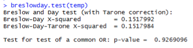
For the boy scout example, the Breslow-Day statistic is 0.15 with df = 2, p-value = 0.93. We do NOT have sufficient evidence to reject the model of homogeneous associations. Furthermore, the evidence is strong that associations are very similar across different levels of socioeconomic status.
The expected odds ratio for each table are: \(\hat{\theta}_{BD(high)}=1.20\approx \hat{\theta}_{BD(mild)}=0.89\approx \hat{\theta}_{BD(low)}=1.02\)
In this case, the common odds estimate from CMH test is a good estimate of the above values, i.e., common OR=0.978 with 95% confidence interval (0.597, 1.601).
Of course, this was to be expected for this example, since we already concluded that the conditional independence model fits well, and the conditional independence model is a special case of the homogeneous association model.
We will see more about these models and functions in both R and SAS in the upcoming lessons.
Example - Graduate Admissions
Next, let's see how this works for the Berkeley admissions data. Recall that we set \(X=\) sex, \(Y=\) admission status, and \(Z=\) department. The question of bias in admission can be approached with two tests characterized by the following null hypotheses: 1) sex is marginally independent of admission, and 2) sex and admission are conditionally independent, given department.
For the test of marginal independence of sex and admission, the Pearson test statistic is \(X^2 = 92.205\) with df = 1 and p-value approximately zero. All the expected values are greater than five, so we can rely on the large sample chi-square approximation to conclude that sex and admission are significantly related. More specifically, the estimated odds ratio, 0.5423, with 95% confidence interval (0.4785, 0.6147) indicates that the odds of acceptance for males are about two times as high as that for females.
What about this relationship viewed within a particular department? The CMH test statistic of 1.5246 with df = 1 and p-value = 0.2169 indicates that sex and admission are not (significantly) conditionally related, given department. The Mantel-Haenszel estimate of the common odds ratio is \(0.9047=1/1.1053\) with 95% CI \((0.7719, 1.0603)\). However, the Breslow-Day statistic testing for the homogeneity of the odds ratio is 18.83 with df = 5 and p-value = 0.002!