13: Course Summary-Hide
13: Course Summary-HideCourse Summary
Overview of probability and inference

(ref: Wasserman(2004))
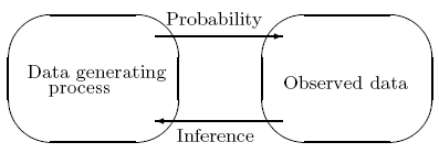
The basic problem we study in probability:
Given a data generating process, what are the properties of the outcomes?
The basic problem of statistical inference:
Given the outcomes, what can we say about the process that generated the data?
For example, given the observed cell counts, what are the true cell probabilities?
Discrete probability & Statistical Inference (Lecture 1 )
- Distributions: Bernoulli, Binomial, Poisson, Multinomial
- Sampling Schemes: Binomial, Poisson, Multinomial, Product-Multinomial, Hypergeometric Sampling
- Estimation: maximum likelihood estimation, concepts of likelihood and loglikelihood
- Confidence intervals
- Hypothesis testing
We applied these three basic inferential problems to significance testing and modeling of one-way, two-way, three-way and k-way tables, and discrete response as a function of both discrete and continuous data.
- Understand the probability structure of contingency tables: marginal and conditional tables, odds, odds-ratios,
- Understand and evaluate how well an observed table of counts corresponds to the sampling scheme model
- Understand the goodness-of-fit concept and compute goodness-of-fit statistics such as Pearson Chi-Square, Deviance,
- Evaluate the lack-of-fit via Pearson and Deviance residuals
- Understand the probability structure of two-way contingency tables: marginal and conditional tables
- Dealing with nominal, ordinal and matched data
- Measuring independence
- Measuring associations: difference of proportions, relative risk, odds, odds-ratios
- Understand the goodness-of-fit concept and compute goodness-of-fit statistics such as Pearson Chi-Square, Deviance, and Pearson and deviance residuals.
- Measures of linear trend, Pearson correlation, Cochran-Mantel-Heanszel, McNemar’s test, Cohen’s Kappa
- Understand the basic concept of exact inference
- Understand the probability structure of two-way contingency tables: marginal and conditional (partial) tables
- Measuring independence and associations: marginal and conditional odds ratios, Cochran-Mantel-Heanzel test, Breslow-Day statistic
- Various models of independence and associations: complete independence, conditional independence, joint independence, homogeneous associations, saturated model
- Understand the goodness-of-fit concept and compute goodness-of-fit statistics such as Pearson Chi-Square, Deviance, and Pearson and deviance residuals with above models
- Simpson’s paradox
- Graphical representation of the models
- Discrete response as a function of both categorical and continuous predictors.
- Fitting and evaluating the model
- Model diagnostics
- Overdispersion
- ROC
- Loglinear-Logit link
- Intro to GLMs
Forming Logits
Basline-Logit Model
Adjacent Logit Model
Proportional Odds Cumulative Logit Model
Introduction to Generalized Linear Model (GLM)
Poisson Regression for Count Data
Poisson Regression for Rate Data
Negative Binomial Model – an alternative to Poisson Regression when data are more dispersed
When discussing models, we need to keep in mind
- Objective
- Model structure (e.g. variables, formula, equation)
- Model assumptions
- Parameter estimates and interpretation
- Model fit (e.g. goodness-of-fit tests and statistics)
- Model selection
- Two-way log-linear models
- Three-way log-linear models
- Sparse Data: sampling and structural zeros, modeling incomplete tables
- Ordinal Data: Linear by linear association model, Association model
- Dependent Samples: Quasi-independence model, Symmetry, Marginal homogeneity, Quasi-symmetry
Other modeling relevant to categorical data are
- Latent Class Models
- Structural Equation Modeling
- General Estimating Equations (GEE) – semiparametric methods for modeling longitudinal data; with PROC GENMOD use the repeated statement
- Nonlinear Mixed Effects Model (NLME) – a parametric alternative to GEE; can use PROC NLMIXED
- Bayesian Modeling – Bayesian inference is possible by Markov Chain Monte Carlo (MCMC) by using MLWin or WinBugs. See an article at http://www.stat.ufl.edu/~aa/cda/bayes.pdf or Bayesian Models for Categorical Data by Peter Congdon, John Wiley Sons (2005).
- etc... (there are many more types of models!)
Course Summary
Review of Model Selection
Ref. Ch. 9 (Agresti), and more advanced topics on model selection with ordinal data are in Sec. 9.4 and 9.5.
One response variable:
- The logit models can be fit directly and are simpler because they have fewer parameters than the equivalent loglinear model.
- If the response variable has more than two levels, you can use a polytomous logit model.
- If you use loglinear models, the highest-way associations among the explanatory variables should be included in all models.
- Whether you use logit or loglinear formulations, the results will be the same regardless of which formulation you use.
Two or more response variables:
- Use loglinear models because they are more general.
Model selection strategies with Loglinear models
- Determine if some variables are responses and some explanatory. Include associations terms for the explanatory variables in the model. Focus your model search on models that relate the responses to explanatory variables.
- If a margin is fixed by design, included the appropriate term in the loglinear model (to ensure that the marginal fitted values from the model equal to observed margin).
- Try to determine the level of complexity that is necessary by fitting models with
- marginal/main effects only
- all 2way associations
- all 3way associations, etc....
- all highest-way associations.
- Backward elimination strategy (analogous to one discussed for logit models) or a stepwise procedure (be careful in using computer algorithms; you are better off doing likelihood ratio tests, e.g. blue collar data, or a 4-way table handout from Fienberg on detergent use).
Classes of loglinear models:
- loglinear models
- hierarchical loglinear models
- graphical loglinear models
- decomposable loglinear models
- conditional independence models
Introduction to Graphical Models
References for Causal Inference