CASE STUDIES
CASE STUDIESThere are three Case Studies that are presented here in conjunction with the STAT 504 online materials.
- The Penn State Ice Cream Study
- Stress and Smoking Study
- Water Level Study
All three of these feature Dr. William Harkness, Professor Emeritus of Statistics giving a video interview about each of these three cases. SAS code, datasets and other materials related to these cases are presented as the case is discussed. Dr. Harkness has taught STAT 504 in residence for many semesters.
Use the links, left below, to access these pages.
CASE STUDY: Stress and Smoking
CASE STUDY: Stress and SmokingOverview
Overview
 For many people who smoke, the most natural thing to do in the midst of a stressful situation is to reach for a cigarette. Many smokers will explain that smoking helps them to relax and relieves their feeling of stress. Their adamant belief that this truly works has introduced the question of whether smoking does indeed relieved the amount of stress perceived by a smoker. The goal of this study was to investigate the relationship between smoking and the amount of recent life stress perceived, using some other variables such as age, and gender as independent (or explanatory) variables or covariates. Stress is a dependent response variable at three levels. Smoking can be viewed as either independent or independent categorical variable at three levels, and age (3 levels) and gender (2 levels) are independent variables (factors) as follows:
Penn State researchers explored the relationship (if any) between four variables in the dataset, stress.txt:
- smoking status (1 = smoker, 2 = quitter, 3 = non-smoker) in column 1,
- gender (1 = male, 2 = female) in column 2,
- age (1 = young, 2 = middle, 3 = old) in column 3, and
- perceived stress level (1 = severe / a lot, 2 = moderate / some, 3 = mild / none) in column 4.
Stress is a "polytomous response" — having three values.
The data can be cross classified as a four-way table.
The relevant SAS programs and data for this case can be found below:
- stress.sas, and
- the dataset, stress.txt.
A couple of things to know about this study ...
A couple of things to know about this study ... Random Zeros
What is the difference between a random zero and a fixed zero? This dataset includes a random zero. Does this impact the analysis of this data? How so? What can you do about this?
The Experimental Design
Does it make a difference how the data is collected? How does the experimental design impact the analysis of the data in this study? Is this something that you should report? How? Why?
In the context of the design of the study, both Age and Gender should be viewed as explanatory variables. The intent of the study was to obtain 50 males and 50 females in each of three age groups, for a total sample size of 300. For whatever reasons, this was not quite accomplished. There were 48 males and from each of the 3 age groups, and 51, 51 and 47 females in the three age groups, so that there were 144 males and 149 females, and 99, 99, and 95 people in the three age groups.
What kinds of questions can be asked?
Given this set of data, what questions could be asked by researchers? Who decides which questions are going to be the focus of the analysis? What if something else comes up that the researcher has not considered? What role should the statistician play? What responsibilities does the statistician have?
In this case study, with both Stress and Smoking treated as responses
- Is there an interaction between the responses Stress and Smoking?
- Does the explanatory variable (factor) Age affect the joint responses or does it affect one response but not the other, or does it affect neither response?
- Does the explanatory variable (factor) Gender affect the joint responses or does it affect one response but not the other, or does it affect neither response?
- Do the two factors interact to affect the responses?
When one of the two variables is a response (say Stress) and the other (say Smoking) is a ‘factor’
- Are there interaction effects—two-way or three-way--among Age, Gender, and Smoking on the response variable?
- Which factors among the three possible affect the response variable?
Exploratory Analysis
Exploratory AnalysisThe Statistical Models
Loglinear Models
What model is the following SAS program investigating? What question is this part of the program stress.sas asking?
Probably more interesting is to see the effects of both gender and age on stress (later in the same program) ...
In the third type of model where you treat both stress and smoing as responses what happens? Does the problem get more complex? How so?
Polytomous Logisitic Regression Models
Why is this an example of a polytomous logisitic regression?
Could a loglinear model analysis apporach be taken with this data? What are the consequences of this type of an approach with this type of experiment? What happens?
A loglinear approach can be taken for a couple of reasons: (a) to identify possible associations among variables to assist in finding appropriate polytomous models and (b) to illustrate differences between treating variables as responses and factors.
Sample SAS programs (2 responses and 4 responses)
(Again, see the SAS program stress.sas.)
Polytomous Logistic Regression Models with One Response
- Stress on Gender (simplest polytomous model)
- Stress on Smoking, Age, and Gender
- Smoking on Gender
- Smoking on Stress, Age, and Gender
Polytomous Logistic Regression Models with Two Responses
- Stress and Smoking on Gender
- Stress and Smoking on Age
- Stress and Smoking on Gender and Age
How complex can the models get? What are parameter estimates?
How complex can the models get? What are parameter estimates?A Loglinear Approach and Complex Studies
About Parameter Estimates...
What are parameter estimates and how do they aid the analysis of your data?
CASE STUDY: The Ice Cream Study at Penn State
CASE STUDY: The Ice Cream Study at Penn StateOverview
 Penn State University is world famous for its ice cream! Researchers are constantly trying to determine exactly what is most appealing to customers. A study was conducted that focused on what the optimum amount of 'fat' to
have in ice cream. So, they made batches of ice cream with fat content ranging from 0.00 to 0.28 . They randomly had 493 subjects participate in tasting and rating the ice cream, on a scale of 1 (didn't like at all) to 9 (yum yum!), with about 60 or so subjects per fat level. Thus, the response variable is polytomous (9 possible values, on an ordinal scale) and there was one independent variable--fat level, with values 0.00, 0.04, 0.08, ... , 0.28.
Dr. Harkness will give you the inside 'scoop' on what this study is about and where it came from. (pun intended!)
The relevant SAS programs and their outputs can be found below:
For R code see, ice_cream.R
First Steps for Analysis?
First Steps for Analysis?Now that you know a little bit more about what this study involves ... how would you go about addressing this study? What would be your first steps to make some sense of this data and answer the question - what is the optimal fat content level for ice cream?
Dr. Harkness walks through some early steps that you might consider...
The data for the of the study is summarized below as an 8 × 9 two-way table:
You could do an ordinary Chi-square test...
...and here is a copy of the Pearson's ChiSquare test results:
|
***** ANALYSIS OF OBSERVED FREQUENCY TABLE 1 MINIMUM ESTIMATED EXPECTED VALUE IS 1.33 |
||||
| STATISTIC | VALUE | D.F. | PROB. | |
|
PEARSON CHISQUARE |
161.101 | 56 | 0.0000 | |
Conclusion this point...
Clearly, we should not be satisfied with just simply demonstrating that there is a significant difference in the different ice creams with varying fat levels. Don't we want to 'model' the ratings as a function of the fat levels? Won't this be a better way to understand which fat level is optimal? How will Polytomous Logistic Regression help provide us with a more helpful analysis?
Understanding Polytomous Logistic Regression
Understanding Polytomous Logistic RegressionPolytomous Logistic Regression models look at cumulative frequencies.
Table 1: Observed Frequencies
Table 2: Observed Proportions - the observed frequencies converted into percentages
Table 3: Observed Cumulative Proportions - the observed proportions accumulated across rows.
All three of these tables are simply descriptive. Now, we can look at Table 3 where the proportions have been accumulated and look for values that are lower in the higher rating ranges. So, just looking at the data in this was can you determine which ice cream fat level is the best? Can you tell? What are you looking for?
Table 4: Fitted Cumulative Probabilities
What about looking at the Fitted cumulative probabilites in the table above? How does this help you determine which ice cream fat level is the best? Can you tell? What are you looking for?
How does this compare if we just used a simple average of the ratings? Here is a table of the average ratings for each fat level and a plot of a quadratic regression of this data.
|
 |
How does this help us understand this problem? Should you stop here?
The Quadratic Nature of the Responses
Many examples of polytomous regression are linear in nature. Why is this example quadratic in nature?
A Better Regression Approach?
A Better Regression Approach?How well does the regression model work for this data? What if someone did not know about polytomous logistic regression and relied solely on a regression approach to predict optimum fat levels in ice cream? How close does this come?
If we knew nothing about polytomous logisitic regression, how good of a job would ordinary multiple regression do on developing a predictive model for this data? Here is the data, rearranged from the table showing the replications.
When we have replications we need to do a weighted least squares regression, one that is weighted to account for these replications.
Here is the output from Minitab for this calculating a quadratic regression equation of 'Rating' on 'Fat' :
What level of 'Fat' (U) maximizes the average rating? The fitted regression equation is given by
\(Y = 4.2768977 + 36.2380923U - 125.2658465U^2 \)
We can find the maximizing value by differentiating this equation and setting the result equal to 0:
\(\frac{dY}{dU}=36.2380923-250.0531693U=0 \rightarrow \hat{U}=36.2380923 / 250.0531693 =0.144648\)
So, using this least weighted squares regression approach we find that a fat level of 0.144648 yields the highest average rating of participants.
Unpacking the Proportional Odds Model
Unpacking the Proportional Odds ModelHow well does the regression model work for this data? What if someone did not know about polytomous logistic regression and relied solely on a regression approach to predict optimum fat levels in ice cream? How close does this come?
The proportional odds model involves, at first, doing some individual logisitic regressions. Logistic regression involves a binary variable so we will introduce a new indicator variable that will given a value of 1 if the rating is equal to or less than one, and 0 if the rating is two or more. We can now use logistic regression to determine proportion of ratings that are 1 or bigger than 1.
Next, just as before, we will introduce a new indicator variable this time that will given a value of 1 if the rating is equal to or less than two, and 0 if the rating is three or more. We can now perform a second logisitic regression that will provide us with a second fitted model used to determine proportion of ratings that are 2 or bigger than 2.
We will continue performing individual logistic regressions in this same manner for the next higher level of rating and so forth... until I get up to 8.
Here is a link to the details of these 8 fitted logistic regression models with the coefficients for each of these highlighted in yellow. ( Details of Fitted Logistic Regression Models )
What do these individual regressions have to do with determining a proportional odds model?
Let's take a look at all of these coefficients from each of these models in summary...
What does this model assume? Are all of the U's equal? In order to answer this question you need to know something about standard deviations. Here is the standard error reported by SAS for the last model shown above...
How does this help?
Here are the SAS results for the Score Test for the Proportional Odds Assumption. Is this significant? What does this tell us?
Where do we go from here?
(Plot of the 8 models here? Dr. Harkness... Curves that are parrallel...)
How might this relate to an Analysis of Covariance?
Advanced Use of Polytomous Logistic Regression
There is something more that you can do with polytomous logistic regression. What if the categorical variable, instead of being a quantitative explanatory variable such as 'fat level' is in this current study, but was strictly categorical? Is polytomous logistic regression still an appropriate approach?
The Fitted Proportinal Odds Model
The Fitted Proportinal Odds ModelLet's fit the model and in the model we will include a test to see whether the model is valid or not.
Here we have fitted the model and have gotten the Likelihood Ratio provided towards the bottom of the output:
What does this likelihood ration tell us? It tells us that the coefficients U and U2 are not both = 0. There is obviously an effect here...
Now we see that the model has 8 intercepts...
... and a coefficient for U and U2. U the coefficient for the fat level is 33 and the estimated coefficient for the fat level squared is -115.
With these values in hand we need to look back at the theoretical model we are fitting. Here is the theoretical model.
Proportional Odds Model:
\(Ln Prob(Y \le i) / [1 - Prob(Y \le i)]= \alpha_i + \beta_1U + \beta_2U^2 \)
Which we will fit for our coefficients U and U2 as shown below and then ...
Ln Model:
\(Ln Prob(Y \le i | U, U^2) / [1 - Prob(Y \le i | U, U^2)]= \alpha_i + \beta_1U + \beta_2U^2 \)
Fitted Model:
\(Ln Prob(Y \le i | U, U^2) / [1 - Prob(Y \le i | U, U^2)]= \hat{\alpha}_i + 33.08450 - 115.1U^2 \)
Which we can then differentiate and maximize to arrive at a final value of ...
\(\frac{dY}{dU}= 33.0845 - 230.2U^2 = 0 \rightarrow \hat{U} = 33.0845 / 230.2 = 0.14372\)
Reflecting on Polytomous Response
At what point or what number of values on your Likert scale would you hestiate to use regression and feel as though you would have to use polytomous logistic regression?
How about other Likert values that are used? Will the same principle be involved?
CASE STUDY: The Water Level Study
CASE STUDY: The Water Level StudyIntroduction
An Interview with Dr. Harkness
Dr. William Harkness provides his own unique introduction in the first part of this series of video interviews about this study.
Case Overview
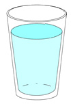 In 1956 Piaget and Imhelder argued that a child needs to construct conceptual systems in order to understand spatial relationships, for example, the Euclidean coordinate system. As part of their research they asked children to draw pictures of vertical and horizontal surfaces. In one task (the water-level task) the child is shown a picture of an upright glass half-filled with water. The child is then shown pictures of tilted glasses and asked to draw a line which represents how the surface of the water would look in these glasses. According to their results, by the age of nine or ten most children have mastered this task. However, later studies have shown that many adults, particularly females, have difficulty with this task.
The robust gender differences observed have had a dramatic impact on the status of Piaget and Imhelder's theory of Euclidean space. If Euclidean space is a construct needed for understanding the relationships between objects in our environment, it is a serious accusation to suggest that large numbers of females lack this construct. Also, if the majority of females do lack this system of reference, it is difficult to explain how they can accomplish tasks such as estimating the trajectories of moving objects while driving an automobile. It seems that the lack of a Euclidean coordinate system would be such a great hindrance that it would be noticeable in everyday life. If the Euclidean system is not used in tasks such as estimating the locations of moving objects, then it is important to discover what skills are facilitated by the Euclidean spatial system.
Some researchers have suggested that many people who fail the water level task may have Euclidean spatial competence, but are affected by specific performance variables and knowledge defects, including
- The ability to draw a horizontal line and the criteria used for passing the task.
- Attempts to draw the water line while the water is moving.
- Understanding and knowledge of relevant physical principles.
- Spatial skills.
The relevant SAS programs and their outputs can be found below:
- water.sas,
- water_level1.sas,
- water_level2.sas,
- water_level3.sas, and
- water_level4.sas.
The Penn State Study
The Penn State StudyDebbie Dalke, a Ph.D. candidate (at Penn State University ) conducted a study to investigate several factors which might provide insight into the gender differences which are so consistently reported in water-level studies. She recruited n = 166 subjects (all college students) from introductory psychology classes. Each subject was given two test booklets. The first was a paper-and-pencil water-level test. This consisted of six drawings of a rectangular glass tipped at one of three different angles on a table top (20, 40, and 60 degree degrees; three tipped to the left and three tipped to the right). A line representing the table top was located beneath the glass (see pictures below). The subjects were told to "Imagine that the glass has water in it and draw a line which represents how the surface of the water will look". A drawing was considered to be correct if the line was within five degrees of true horizontal.
Then each subject was asked "Did you draw the water line as it would look after the glass had come to a complete halt or while it was in motion?" Answers were recorded as a variable MOVING with values "1" if the answer was "complete halt" and "2" if the answer was "moving". Finally, each subject answered questions or performed tasks, in the second booklet, on
- Gravity (5 items - example item)
- Complex Physics (4 items - example item )
- Mental Rotations (Vandenberg's test-6 problems, 2 answers/question).
- Drawing a line inside a triangle; the variable measured was the deviation in degrees from a horizontal line.
- Estimating the intersection of two lines (Bryant's test-3 tasks. Subjects were given 2 points if the "dot" was within 3mm of the intersection, 1 if within 5 mm, and zero otherwise, on each task).
- Drawing a "light-cord" hanging from the ceiling of a trailer going up a hill, slanting either left or right, at angles of either 20 or 40 degrees.
- Drawing a "tree" on the side of a hill, inclined 20, 40, or 60 degrees in both left and right directions. Subject's answers were scored as correct if the drawing in (f) or (g) was within 5 degrees of true vertical.
The Dataset and Variables
The Dataset and VariablesThe datafile, water_level.txt, records 166 observations of the following variables:
The response variable was the outcome on the water-level task. Subjects passed (Y = 1) if they were right on at least 5 out of the 6 water-level drawings and failed (Y = 0) if they missed two or more. There were 10 predictor variables:
SEX: Female (1), Male (2).
GRAVITY: Number of gravity tasks answered correctly.
BRYANT: Total Score on Bryant's test -0, 1, 2, 3, 4.
VANDER: Total number of correct answers (0, 1, …, 12)
TRIANGLE: Score on the triangle task -0, 1, … (degrees from horizontal).
TRAILER: Total Score on the trailer test -0, 1, 2, 3, 4.
TREE: Total Score on the tree drawings -0, 1, …, 8.
COMPHYS: Number of Complex Physics questions answered correctly.
MOVING: Values as given above.
In addition, two other variables, derived from these, will be used:
TOTPHYS: Sum of COMPHYS and GRAVITY-VALUES ARE 0, 1, 2, …, 9.
TOTAL: Sum of TOTPHYS , VANDER, TRIANGLE, BRYANT, TRAILER, AND TREE.
The variables SEX and MOVING are class variables and the rest are quantitative.
Going About Explaining Gender Differences
Can we use logistic regression to address questions like "If a subject is a female and answers all five of the gravity questions correctly, what is the chance (probability) that she passes the water-level task?" Also, ask questions like
- Which set of predictor variables do the best job of predicting the outcome on the water-level task?
- If we "control" or "adjust" for overall knowledge about physics (TOTPHYS), spatial ability as measured by the test on Mental Rotations (VANDER) and performance on a task akin to the water-level one, for example, TREE, does the observed difference between the sexes vanish?
Exploratory Analysis - 1
Exploratory Analysis - 1Test the Equality of Two Proportions
The SAS program water.sas provides the following frequency table (and others) of the water level study data:

Why was the passing rate so low? What factors affect passing?
In the past statisticians have used ordinary regression when experiments involved categorical data. Wouldn't it be interesting to see how bad an ordinary regression analysis is compared to using logistic regression?
First we could run a Pearson Chi-Square to test the equality of two proportions. Our hypothesis at this stage is that the proportion of males passing is the same as the proportion of females that passed. As the frequency table above reports, the observed percentage of females who passed is 29.91% and the observed proportion of males who passed is 64.41%.
When we look at the Pearson Chi-squared test of equality of two proportions we would find a Chi-Square value of 18.562, p-value = 0.000.
This is highly significant, (because the p-value is also < 0.05), so, we reject the hypothesis that the proportions passing are the same for females and males.
Exploratory Analysis - 2
Exploratory Analysis - 2Logisitic Regression with a Qualitatitve (Categorical) Variable
Logistic Regression
Logistic Regression of Pass/Fail
Let's use logistic regression to test passing versus failing. We can test the model:
\(\text{Model: } ln\{\pi(sex)/[1-\pi(sex)]\}=\beta_0+\beta_1 \ast (sex)=\begin{array} {l @{\quad,\quad} l}
\beta_0+\beta_1 & \text{for females}\\ \beta_0 & \text{for males} \end{array} \)
and use the SAS program water_level1.sas below. This program uses the frequency counts for both sex and whether they passed the test:
What do the results indicate? In this case we can see that in testing the following:
H0: No Sex effect or H0 : β1 = 0 vs. the alternative Ha : β1 ≠ 0
the Likelihood Ratio, G2 = 18.6578 ...
Therefore, we must reject null hypothesis - no sex effect - and conclude that there is statictically significant difference between females and males in proportion passing the test.
We can fit the model using these values from the output:
where the
fitted logit(females) = 0.5931 - 1.4446 = -0.8515 for females
fitted logit(males) = 0.5931 for males
The odds ratio (males vs. females) = s-1.4446 = 0.236
The odds ratio = (38)(75)/(21)(32) = 4.24 = s-1.4446
Exploratory Analysis - 3
Exploratory Analysis - 3Logistic Regression with a Quantitative Variable
(Pass/Fail on x = Gravity)
Now, let's see if the quantitative variable gravity has any effect on the passing or failing and test: Model: \( ln \pi(x)/[1-\pi(x)]\). We can use the SAS program water_level2.sas below to do this.
Our hypothesis is:
H0 : No gravity effect or H0 : β1 = 0 vs. the alternative Ha : β1 ≠ 0
The output from the program provides us with a G2 = 42.1765...
Therefore, we must reject H0, there is no gravity effect and conclude there is a statistically significant difference between the gravity score and the proportion passing the task.
We can fit the model using the values from the output:
such that the:
Fitted Model: Estimated logit[π (x)] = -2.8156 + 0.7998x
Here is the Odds Ratio Estimates output:
which in a sense tell us that the odds of passing the water level task increase by 2.225 for each additional right answer on gravity.
If we take the observed and fitted proportions that are given (below) in the output:
we have added a couple of lines of code to our program so that SAS displays a graph of the observed and fitted(phat) proportions, below:
How does the 'fit' look?
Exploratory Analysis - 4
Exploratory Analysis - 4Logistic Regression with 1 Qualitative and 1 Quantitative Variable
(Pass/Fail on x = Sex and Gravity)
First, let's perform logisitic regression of passing or failing the test on the variables sex and gravity using the following models:
Model: logit [π(sex, gravity)] = β0+ β1* (sex) + β2*gravity
(β0+ β1) + β2*gravity, for females, and
(β0+ 2β1) + β2*gravity, for males
We can use the first PROC LOGISTIC procedure in the following SAS program water_level3a.sas to run this.
First we are testing:
H0 : sex and gravity together do not affect passing the water level task, or
H0 : β1 = β2 = 0 vs. Ha: at least one of the parameters is not 0.
We can see by the output that results:

that G2 = 50.9766 = LRT .
We will conclude that the logistic regression of pass/fail on sex and gravity is not statistically significant.
The estimated logit(sex, gravity) = -4.1676 + 1.1220sex + 0.7404gravity.
Note that sex is coded as 1 for females and 2 for males.
No Gravity Effect, Adjusted for Sex?
If we were to test the hypothesis that there is no gravity effect, adjusted for 'sex', we would calculate the change in G2 for the model with both variables included and the model with only sex included (see water_level1.sas output). For instance,
G2 (sex, gravity) - G2(sex) = 50.9766 - 42.1765 = 8.801.
Or, we could calculate the change in the 2loglikelihood:
-2ln(sex) - [-2ln(sex, gravity)] = 183.859 - 175.059 = 8.800
Compare this with the Wald chi-square of 8.6117.
No Sex Effect, Adjusted for Gravity?
Now let's test the hypothesis that there is no sex effect, adjusted for the gravity score. We would calculate the change in G2 for the model with both variables included and the model with only gravity (see water_level2.sas output).
G2 (sex, gravity) - G2(gravity) = 50.9766 - 18.6568 = 32.319.
Or, we could calculate the change in the 2loglikelihood:
-2ln(gravity) - [-2ln(sex, gravity)] = 207.478 - 175.059 = 32.419
Now, how does this compare this with the Wald chi-square of 25.4979?
Predicted values and confidence limits for population proportions:
Edited fitted values are given below.
edited values here...
A plot of phat vs. gravity for females and males is given in the graph.
graph here...
Logistic Regression of Pass/Fail on Sex, Gravity and Sex* Gravity (Interaction Model)
Here our model is:
Model: logit [π(sex, gravity)] = β0+ β1* (sex) + β2*gravity + β3*(sex*gravity)
(β0+ β1) + (β2 + β3)gravity, for females, and
(β0+ 2β1) + (β2 + 2β3)gravity, for males
SAS output:
Exploratory Analysis - 5
Exploratory Analysis - 5Binary Logisitic Regression on a Categorical Variable with 3 Values
(Pass/Fail on x = 'Sex Move')
Binary Logistic Regression
What we have looked at thus far in this exploratory analysis were 2 × 2 tables. Now we are going to move to 2 × 3 tables.
First we will tally the discrete variable Moving. Moving was coded as 1 if the person said that the glass was not moving when they drew the line, and 2 if it was. 29 out of the 166 subjects said that the glass was moving.
|
Moving
|
Count |
|
1
|
137
|
|
2
|
29
|
|
N = 166
|
Now we will create a new variable called 'sexMove' as follows: Gender is coded 0 = female and 1 = male. Moving was coded as 1 if the person said that the glass was not moving when they drew the line, and 2 if it was. We will let the combined 'Gender by Move' = 10*Gender + Move.
According to the dataset 79 females said the glass was not moving, 28 females said the glass was moving. 58 of the males said the glass was not moving and only 1 male said the glass was moving
|
Female, Not moving
|
79 |
|
Female, Moving
|
28
|
|
Male, Not moving`
|
58
|
|
Male, Moving
|
1
|
|
N = 166
|
For the purposes of this analysis we will combine the last two rows and label it Male such that this new variable, SexMove, will have 3 values, 1, 2 and 3.
|
Value
|
Description
|
Count
|
|
1
|
if the person is female and said the glass was not moving |
79
|
|
2
|
if the person is female and said the glass was moving |
28
|
|
3
|
if the person is male |
59
|
We can run the binary logisitic regression using the SAS program ???
SAS program image here...
SAS output and discussion here ...
Conclusion
There is a very highly significant difference in the proportions of persons passing for the three values of SexMove. Only 7.14% of females who said the glass was moving passed the water level task. 37.97% of the females who said the glass was not moving passed, and 64.41% of the males passed the task. Only one male out of 59 said the glass was moving compared to 28 out of 107 females.
Exploratory Analysis - 6
Exploratory Analysis - 6Backward Elimination & Stepwise Selection Procedures
We will begin here by using two subset selection procedures in SAS Proc Logistic for choosing variables related to the response:
- Backward elimination
- Stepwise selection
Which Model Should I Fit?
Take a look at this SAS program (water_level3.sas):
The data are input, the variables identified and then the PROC LOGISTIC procedure is called specifying a model where Y (subjects passed, 1 or failed, 0) is the response. Notice, highlighted in purple, the use of the word 'backward' and 'stepwise' to specify the two different subset selection procedures.
Backward Elimination
In the output, the procedure begins by entering all of the variables:
and then one by one the variables are removed...


Each time the model is re-fit until at the end of the procedure the note below is reported along with the four variables that were removed from the model fit.
Directly after this the procedure lists the variables that are retained in the model as their p-values and all < 0.05:
along with the coefficients that make up the fitted model.
Stepwise Selection
This procedure takes the opposite approach beginning with one variable and subsequently adding additional variables, on at a time, to the model, fitting it each time.

until at the end of the procedure the following note is given:

and a summary list of the variables that remain in the model is displayed:
Odds Ratio Estimates
If we look at the Odds Ratio Estimates for both procedures:
Backward Elimination
Stepwise Selection
The two procedures each selected 6 variables with 5 in common; backward elimination chose ‘gravity’ while stepwise chose ‘totphysics’. The odds ratio and confidence interval estimates are quite close for all variables.
Furthermore, neither model includes the variable ‘sex’. We conclude that adjusted for these 6 independent variables ‘sex’ does not affect passing/failing.
This handout covers this information as well: WaterStudyModelSelection.pdf