Now that you know a little bit more about what this study involves ... how would you go about addressing this study? What would be your first steps to make some sense of this data and answer the question - what is the optimal fat content level for ice cream?

Dr. Harkness walks through some early steps that you might consider...

The data for the of the study is summarized below as an 8 × 9 two-way table:

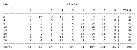
You could do an ordinary Chi-square test...

...and here is a copy of the Pearson's ChiSquare test results:

Conclusion this point...

Clearly, we should not be satisfied with just simply demonstrating that there is a significant difference in the different ice creams with varying fat levels. Don't we want to 'model' the ratings as a function of the fat levels? Won't this be a better way to understand which fat level is optimal? How will Polytomous Logistic Regression help provide us with a more helpful analysis?

Polytomous Logistic Regression models look at cumulative frequencies.

Table 1: Observed Frequencies

Table 2: Observed Proportions - the observed frequencies converted into percentages

Table 3: Observed Cumulative Proportions - the observed proportions accumulated across rows.

All three of these tables are simply descriptive. Now, we can look at Table 3 where the proportions have been accumulated and look for values that are lower in the higher rating ranges. So, just looking at the data in this was can you determine which ice cream fat level is the best? Can you tell? What are you looking for?

Table 4: Fitted Cumulative Probabilities

What about looking at the Fitted cumulative probabilites in the table above? How does this help you determine which ice cream fat level is the best? Can you tell? What are you looking for?

How does this compare if we just used a simple average of the ratings? Here is a table of the average ratings for each fat level and a plot of a quadratic regression of this data.

Fat Level Mean .00 3.81 .04 6.03 .08 6.71 .12 6.81 .16 6.55 .20 6.44 .24 5.44 .28 4.94

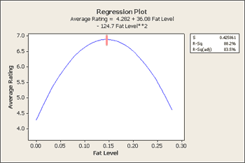How does this help us understand this problem? Should you stop here?

The Quadratic Nature of the Responses

Many examples of polytomous regression are linear in nature. Why is this example quadratic in nature?

How well does the regression model work for this data? What if someone did not know about polytomous logistic regression and relied solely on a regression approach to predict optimum fat levels in ice cream? How close does this come?

If we knew nothing about polytomous logisitic regression, how good of a job would ordinary multiple regression do on developing a predictive model for this data? Here is the data, rearranged from the table showing the replications.

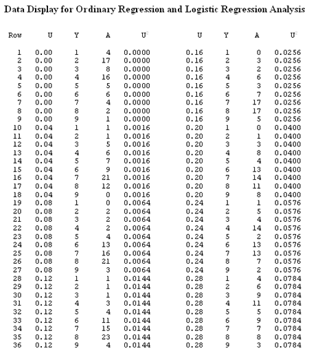
When we have replications we need to do a weighted least squares regression, one that is weighted to account for these replications.

Here is the output from Minitab for this calculating a quadratic regression equation of 'Rating' on 'Fat' :

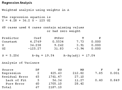
What level of 'Fat' (U) maximizes the average rating? The fitted regression equation is given by

\(Y = 4.2768977 + 36.2380923U - 125.2658465U^2 \)

We can find the maximizing value by differentiating this equation and setting the result equal to 0:

\(\frac{dY}{dU}=36.2380923-250.0531693U=0 \rightarrow \hat{U}=36.2380923 / 250.0531693 =0.144648\)

So, using this least weighted squares regression approach we find that a fat level of 0.144648 yields the highest average rating of participants.

How well does the regression model work for this data? What if someone did not know about polytomous logistic regression and relied solely on a regression approach to predict optimum fat levels in ice cream? How close does this come?

The proportional odds model involves, at first, doing some individual logisitic regressions. Logistic regression involves a binary variable so we will introduce a new indicator variable that will given a value of 1 if the rating is equal to or less than one, and 0 if the rating is two or more. We can now use logistic regression to determine proportion of ratings that are 1 or bigger than 1.

Next, just as before, we will introduce a new indicator variable this time that will given a value of 1 if the rating is equal to or less than two, and 0 if the rating is three or more. We can now perform a second logisitic regression that will provide us with a second fitted model used to determine proportion of ratings that are 2 or bigger than 2.

We will continue performing individual logistic regressions in this same manner for the next higher level of rating and so forth... until I get up to 8.

Here is a link to the details of these 8 fitted logistic regression models with the coefficients for each of these highlighted in yellow. ( Details of Fitted Logistic Regression Models )

What do these individual regressions have to do with determining a proportional odds model?

Let's take a look at all of these coefficients from each of these models in summary...

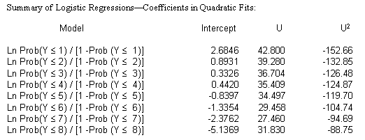
What does this model assume? Are all of the U's equal? In order to answer this question you need to know something about standard deviations. Here is the standard error reported by SAS for the last model shown above...

How does this help?

Here are the SAS results for the Score Test for the Proportional Odds Assumption. Is this significant? What does this tell us?

Where do we go from here?

(Plot of the 8 models here? Dr. Harkness... Curves that are parrallel...)

How might this relate to an Analysis of Covariance?

Advanced Use of Polytomous Logistic Regression

There is something more that you can do with polytomous logistic regression. What if the categorical variable, instead of being a quantitative explanatory variable such as 'fat level' is in this current study, but was strictly categorical? Is polytomous logistic regression still an appropriate approach?

Let's fit the model and in the model we will include a test to see whether the model is valid or not.

Here we have fitted the model and have gotten the Likelihood Ratio provided towards the bottom of the output:

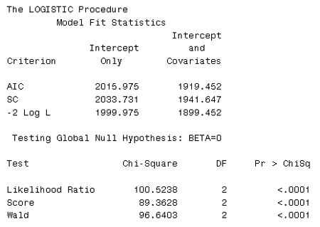
What does this likelihood ration tell us? It tells us that the coefficients U and U² are not both = 0. There is obviously an effect here...

Now we see that the model has 8 intercepts...

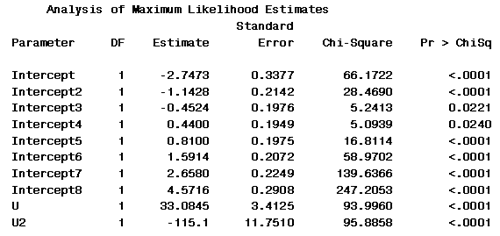
... and a coefficient for U and U². U the coefficient for the fat level is 33 and the estimated coefficient for the fat level squared is -115.

With these values in hand we need to look back at the theoretical model we are fitting. Here is the theoretical model.

Proportional Odds Model:

\(Ln Prob(Y \le i) / [1 - Prob(Y \le i)]= \alpha_i + \beta_1U + \beta_2U^2 \)

Which we will fit for our coefficients U and U² as shown below and then ...

Ln Model:

\(Ln Prob(Y \le i | U, U^2) / [1 - Prob(Y \le i | U, U^2)]= \alpha_i + \beta_1U + \beta_2U^2 \)

Fitted Model:

\(Ln Prob(Y \le i | U, U^2) / [1 - Prob(Y \le i | U, U^2)]= \hat{\alpha}_i + 33.08450 - 115.1U^2 \)

Which we can then differentiate and maximize to arrive at a final value of ...

\(\frac{dY}{dU}= 33.0845 - 230.2U^2 = 0 \rightarrow \hat{U} = 33.0845 / 230.2 = 0.14372\)

Reflecting on Polytomous Response

At what point or what number of values on your Likert scale would you hestiate to use regression and feel as though you would have to use polytomous logistic regression?

How about other Likert values that are used? Will the same principle be involved?