4.1 - Comparing Distribution Types

Univariate Normal Distributions

Before defining the multivariate normal distribution we will visit the univariate normal distribution. A random variable X is normally distributed with mean \(\mu\) and variance \(\sigma^{2}\) if it has the probability density function of X as:

\(\phi(x) = \frac{1}{\sqrt{2\pi\sigma^2}}\exp\{-\frac{1}{2\sigma^2}(x-\mu)^2\}\)

This result is the usual bell-shaped curve that you see throughout statistics. In this expression, you see the squared difference between the variable x and its mean, \(\mu\). This value will be minimized when x is equal to \(\mu\). The quantity \(-\sigma^{-2}(x - \mu)^{2}\) will take its largest value when x is equal to \(\mu\) or likewise since the exponential function is a monotone function, the normal density takes a maximum value when x is equal to \(\mu\).

The variance \(\sigma^{2}\) defines the spread of the distribution about that maximum. If \(\sigma^{2}\) is large, then the spread is going to be large, otherwise, if the \(\sigma^{2}\) value is small, then the spread will be small.

As shorthand notation we may use the expression below:

\(X \sim N(\mu, \sigma^2)\)

indicating that X is distributed according to (denoted by the wavey symbol 'tilde') a normal distribution (denoted by N), with mean \(\mu\) and variance \(\sigma^{2}\).

Multivariate Normal Distributions

If we have a p x 1 random vector \(\mathbf{X} \) that is distributed according to a multivariate normal distribution with a population mean vector \(\mu\) and population variance-covariance matrix \(\Sigma\), then this random vector, \(\mathbf{X} \), will have the joint density function as shown in the expression below:

\(\phi(\textbf{x})=\left(\frac{1}{2\pi}\right)^{p/2}|\Sigma|^{-1/2}\exp\{-\frac{1}{2}(\textbf{x}-\mathbf{\mu})'\Sigma^{-1}(\textbf{x}-\mathbf{\mu})\}\)

\(| \Sigma |\) denotes the determinant of the variance-covariance matrix \(\Sigma\) and \(\Sigma^{-1}\)is just the inverse of the variance-covariance matrix \(\Sigma\). Again, this distribution will take maximum values when the vector \(\mathbf{X} \) is equal to the mean vector \(\mu\), and decrease around that maximum.

If p is equal to 2, then we have a bivariate normal distribution and this will yield a bell-shaped curve in three dimensions.

The shorthand notation, similar to the univariate version above, is

\(\mathbf{X} \sim N(\mathbf{\mu},\Sigma)\)

We use the expression that the vector \(\mathbf{X} \) 'is distributed as' multivariate normal with mean vector \(\mu\) and variance-covariance matrix \(\Sigma\).

Some things to note about the multivariate normal distribution:

The following term appearing inside the exponent of the multivariate normal distribution is a quadratic form:
\((\textbf{x}-\mathbf{\mu})'\Sigma^{-1}(\textbf{x}-\mathbf{\mu})\)

This particular quadratic form is also called the squared Mahalanobis distance between the random vector x and the mean vector \(\mu\).
If the variables are uncorrelated then the variance-covariance matrix will be a diagonal matrix with variances of the individual variables appearing on the main diagonal of the matrix and zeros everywhere else:
\(\Sigma = \left(\begin{array}{cccc}\sigma^2_1 & 0 & \dots & 0\\ 0 & \sigma^2_2 & \dots & 0\\ \vdots & \vdots & \ddots & \vdots\\ 0 & 0 & \dots & \sigma^2_p \end{array}\right)\)

Multivariate Normal Density Function

In this case the multivariate normal density function simplifies to the expression below:

\(\phi(\textbf{x}) = \prod_{j=1}^{p}\frac{1}{\sqrt{2\pi\sigma^2_j}}\exp\{-\frac{1}{2\sigma^2_j}(x_j-\mu_j)^2\}\)

Note! The product term, given by 'capital' pi, (\(Π\)), acts very much like the summation sign, but instead of adding we multiply over the elements ranging from j=1 to j=p. Inside this product is the familiar univariate normal distribution where the random variables are subscripted by j. In this case, the elements of the random vector, \(\mathbf { X } _ { 1 }, \mathbf { X } _ { 2 , \cdots } \mathbf { X } _ { p }\), are going to be independent random variables.
We could also consider linear combinations of the elements of a multivariate normal random variable as shown in the expression below:
\(Y = \sum_{j=1}^{p}c_jX_j =\textbf{c}'\textbf{X}\)

Note! To define a linear combination, the random variables \(X_{j}\) need not be uncorrelated. The coefficients \(c_{j}\) are chosen arbitrarily, specific values are selected according to the problem of interest and so are influenced very much by subject matter knowledge. Looking back at the Women's Nutrition Survey Data, for example, we selected the coefficients to obtain the total intake of vitamins A and C.

Now suppose that the random vector X is multivariate normal with mean \(\mu\) and variance-covariance matrix \(\Sigma\).

\(\textbf{X} \sim N(\mathbf{\mu},\Sigma)\)

Then Y is normally distributed with mean:

\(\textbf{c}'\mathbf{\mu} = \sum_{j=1}^{p}c_j\mu_j\)

and variance:

\(\textbf{c}'\Sigma \textbf{c} =\sum_{j=1}^{p}\sum_{k=1}^{p}c_jc_k\sigma_{jk}\)

See the previous lesson to review the computation of the population mean of a linear combination of random variables.

In summary, Y is normally distributed with mean c transposed \(\mu\) and variance c transposed times \(\Sigma\) times c.

\(Y \sim N(\textbf{c}'\mathbf{\mu},\textbf{c}'\Sigma\textbf{c})\)

As we have seen before, these quantities may be estimated using sample estimates of the population parameters.

Other Useful Results for the Multivariate Normal

For variables with a multivariate normal distribution with mean vector \(\mu\) and covariance matrix \(\Sigma\), some useful facts are:

Every single variable has a univariate normal distribution. Thus we can look at univariate tests of normality for each variable when assessing multivariate normality.
Any subset of the variables also has a multivariate normal distribution.
Any linear combination of the variables has a univariate normal distribution.
Any conditional distribution for a subset of the variables conditional on known values for another subset of variables is a multivariate distribution. The full meaning of this statement will be clear after Lesson 6.

Example 4-1 - Linear Combination of the Cholesterol Measurements

Measurements were taken on n heart-attack patients on their cholesterol levels. For each patient, measurements were taken 0, 2, and 4 days following the attack. Treatment was given to reduce cholesterol levels. The sample mean vector is:

Variable	Mean
X₁ = 0-Day	259.5
X₂ = 2-Day	230.8
X₃ = 4-Day	221.5

The covariance matrix is

	0-Day	2-Day	4-day
0-Day	2276	1508	813
2-Day	1508	2206	1349
4-Day	813	1349	1865

Suppose that we are interested in the difference \(X _ { 1 } - X _ { 2 }\), the difference between the 0-day and the 2-day measurements. We can write the linear combination of interest as

\(\textbf{a}'\textbf{x}= \left(\begin{array}{ccc}1 & -1 & 0 \end{array}\right)
\left(\begin{array}{c}x_1\\ x_2\\ x_3 \end{array}\right)\)

The mean value for the difference is

\begin{align} &=\left(\begin{array}{ccc}1 & -1 & 0 \end{array}\right)\left(\begin{array}{c}259.5\\230.8\\221.5 \end{array}\right)\\ & = 28.7 \end{align}

The variance is

\begin{align} &=\left(\begin{array}{ccc}1 & -1 & 0 \end{array}\right) \left(\begin{array}{ccc}2276 & 1508 & 813\\ 1508 & 2206 & 1349\\ 813 & 1349 & 1865 \end{array}\right) \left(\begin{array}{c}1\\-1\\0 \end{array}\right)\\&= \left(\begin{array}{ccc}768 & -698 & -536 \end{array}\right)\left(\begin{array}{c}1\\-1\\0 \end{array}\right) \\ &= 1466 \end{align}

If we assume the three measurements have a multivariate normal distribution, then the distribution of the difference \(X _ { 1 } - X _ { 2 }\) has a univariate normal distribution.

4.2 - Bivariate Normal Distribution

Bivariate Normal Distribution

To further understand the multivariate normal distribution it is helpful to look at the bivariate normal distribution. Here our understanding is facilitated by being able to draw pictures of what this distribution looks like.

We have just two variables, \(X_{1}\) and \(X_{2}\), and these are bivariately normally distributed with mean vector components \(\mu_{1}\) and \(\mu_{2}\) and variance-covariance matrix shown below:

\(\left(\begin{array}{c}X_1\\X_2 \end{array}\right) \sim N \left[\left(\begin{array}{c}\mu_1\\ \mu_2 \end{array}\right), \left(\begin{array}{cc}\sigma^2_1 & \rho \sigma_1\sigma_2 \\ \rho\sigma_1\sigma_2 & \sigma^2_2 \end{array}\right)\right]\)

In this case, we have the variances for the two variables on the diagonal and on the off-diagonal, we have the covariance between the two variables. This covariance is equal to the correlation times the product of the two standard deviations. The determinant of the variance-covariance matrix is simply equal to the product of the variances times 1 minus the squared correlation.

\(|\Sigma| = \sigma^2_1\sigma^2_2(1-\rho^2)\)

The inverse of the variance-covariance matrix takes the form below:

\(\Sigma^{-1} = \dfrac{1}{\sigma^2_1\sigma^2_2(1-\rho^2)} \left(\begin{array}{cc}\sigma^2_2 & -\rho \sigma_1\sigma_2 \\ -\rho\sigma_1\sigma_2 & \sigma^2_1 \end{array}\right)\)

Joint Probability Density Function for Bivariate Normal Distribution: Substituting in the expressions for the determinant and the inverse of the variance-covariance matrix we obtain, after some simplification, the joint probability density function of (\(X_{1}\), \(X_{2}\)) for the bivariate normal distribution as shown below:; \(\phi(x_1,x_2) = \dfrac{1}{2\pi\sigma_1\sigma_2\sqrt{1-\rho^2}}\exp\{-\dfrac{1}{2(1-\rho^2)}\left[\left(\dfrac{x_1-\mu_1}{\sigma_1}\right)^2-2\rho \left(\dfrac{x_1-\mu_1}{\sigma_1}\right) \left(\dfrac{x_2-\mu_2}{\sigma_2}\right) + \left(\dfrac{x_2-\mu_2}{\sigma_2}\right)^2 \right]\}\)

The following three plots are plots of the bivariate distribution for the various values for the correlation row.

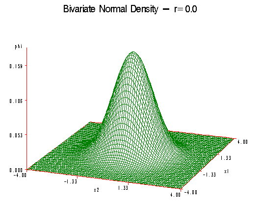
The first plot shows the case where the correlation \(\rho\) is equal to zero. This special case is called the circular normal distribution. Here, we have a perfectly symmetric bell-shaped curve in three dimensions.

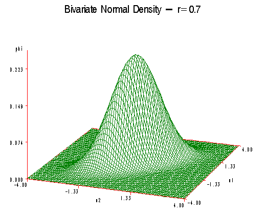
As ρ increases that bell-shaped curve becomes flattened on the 45-degree line. So for \(\rho\) equals 0.7 we can see that the curve extends out towards minus 4 and plus 4 and becomes flattened in the perpendicular direction.

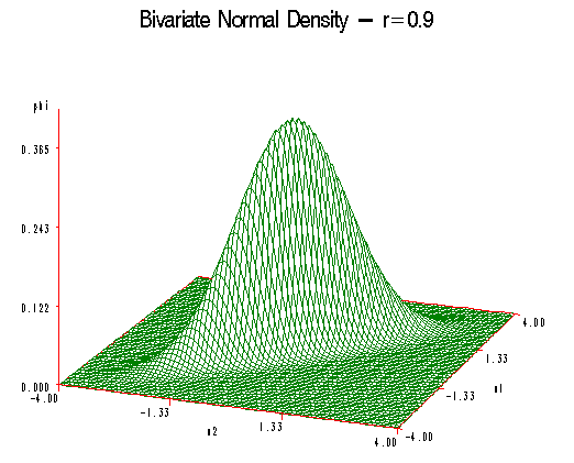
Increasing \(\rho\) to 0.9 the curve becomes broader and the 45-degree line and even flatter still in the perpendicular direction.

These three curves were produced using the SAS program shown below. The desired correlation is specified in the third line of the SAS code (here at 0.9). No other changes are required to run this program. It would be a good idea to try this program for various values of r between -1 and 1 to explore how the shape of the normal distribution varies with the correlation.

Note: In the upper right-hand corner of the code block you will have the option of copying () the code to your clipboard or downloading () the file to your computer.

options ls=78;   /*This sets the max number of lines per page to 78.*/
title "Bivariate Normal Density";   /*This sets a title that will appear on each page of the output until it's changed.*/
%let r=0.9;   /*This defines the macro variable r; it will be referenced with &r throughout the code.*/
data a;   /*This data set defines the coordinates for plotting the bivariate normal pdf. The domain is the square of values between -4 and 4 for both x1 and x2. And phi represents the value of the normal pdf as a function of both x1 and x2.*/
  pi=3.1416;   
  do x1=-4 to 4 by 0.1;   
    do x2=-4 to 4 by 0.1;   
      phi=exp(-(x1*x1-2*&r*x1*x2+x2*x2)/2/(1-&r*&r))/2/pi/sqrt(1-&r*&r);   
      output;   
    end;   
  end;   
  run;   
proc g3d;   /*This plots in 3d the bivariate pdf for the variables x1, x2, and phi defined in the data set "a" above. The viewing angle is determined by the 'rotate' option.*/
  plot x1*x2=phi / rotate=-20;   
  run;

Note! This code assumes that the variances are both equal to one.

How to Use Minitab to Create Plots of the Bivariate Distribution.

You will need the formula that is found in the downloadable text file here: phi_equation_r=0.7.txt.

To plot a bivariate normal density for a given correlation value:

4.3 - Exponent of Multivariate Normal Distribution

Recall the Multivariate Normal Density function below:

\(\phi(\textbf{x}) = \left(\frac{1}{2\pi}\right)^{p/2}|\Sigma|^{-1/2}\exp\{-\frac{1}{2}(\textbf{x}-\mathbf{\mu})'\Sigma^{-1}(\textbf{x}-\mathbf{\mu})\}\)

You will note that this density function, \(\phi(\textbf{x})\), only depends on x through the squared Mahalanobis distance:

\((\textbf{x}-\mathbf{\mu})'\Sigma^{-1}(\textbf{x}-\mathbf{\mu})\)

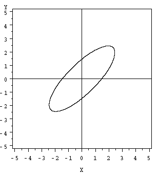
This is the equation for a hyper-ellipse centered at \(\mu\).

For a bivariate normal, where p = 2 variables, we have an ellipse as shown in the plot below:

Ellipse where p=2

Useful facts about the Exponent Component: \( (\textbf{x}-\mathbf{\mu})'\Sigma^{-1}(\textbf{x}-\mathbf{\mu})\)

All values of x such that \( (\textbf{x}-\mathbf{\mu})'\Sigma^{-1}(\textbf{x}-\mathbf{\mu})=c\) for any specified constant value c have the same value of the density \(f(x)\) and thus have an equal likelihood.
As the value of \((\textbf{x}-\mathbf{\mu})'\Sigma^{-1}(\textbf{x}-\mathbf{\mu})\) increases, the value of the density function decreases. The value of \((\textbf{x}-\mathbf{\mu})'\Sigma^{-1}(\textbf{x}-\mathbf{\mu})\) increases as the distance between x and \(\mu\) increases.
The variable \(d^2=(\textbf{x}-\mathbf{\mu})'\Sigma^{-1}(\textbf{x}-\mathbf{\mu})\) has a chi-square distribution with p degrees of freedom.
The value of d ² for a specific observation \(\textbf{x}_j\) is called a squared Mahalanobis distance.

Squared Mahalanobis Distance: \(d^2_j = (\textbf{x}_j-\mathbf{\bar{x}})'\Sigma^{-1}(\textbf{x}_j-\mathbf{\bar{x}})\)

If we define a specific hyper-ellipse by taking the squared Mahalanobis distance equal to a critical value of the chi-square distribution with p degrees of freedom and evaluate this at \(α\), then the probability that the random value X will fall inside the ellipse is going to be equal to \(1 - α\).

\(\text{Pr}\{(\textbf{x}-\mathbf{\mu})'\Sigma^{-1}(\textbf{x}-\mathbf{\mu}) \le \chi^2_{p,\alpha}\}=1-\alpha\)

This particular ellipse is called the \((1 - α) \times 100%\) prediction ellipse for a multivariate normal random vector with mean vector \(\mu\) and variance-covariance matrix \(Σ\).

Using Technology

Example
Example

Calculating Mahalanobis Distance With SAS

SAS does not provide Mahalanobis distance directly, but we can compute them using principal components. The steps are:

Determine the principal components for the correlation matrix of the x-variables.
Standardize the principal component scores so that each principal component has a standard deviation = 1. For each component, this is done by dividing the scores by the square root of the eigenvalue. In SAS, use the STD option as part of the PROC PRINCOMP command to automate this standard deviation.
For each observation, calculate \(d^{2}\) = sum of squared standardized principal components scores. This will equal the squared Mahalanobis distance.

Example - Calculating and Printing Mahalonobis Distances in SAS

Suppose we have four x-variables, called \(x_1 , x_2 , x_3 , x_4\), and they have already been read into SAS. The following SAS code (Download below) will determine standardized principal components and calculate Mahalanobis distances (the printout will include observation numbers). Within the DATA step, the “uss(of prin1-prin4)” function calculates the uncorrected sum of squares for the variables prin1-prin4. This value will be computed for each observation in the “pcout” data set. The result of the DATA step will be a SAS data set named “mahal” that will include the original variables, the standardized principal component scores (named prin1-prin4), and the Mahalanobis distance (named dist2).

Data file: boardstiffness.csv

Note: In the upper right-hand corner of the code block you will have the option of copying () the code to your clipboard or downloading () the file to your computer.

data boards; /*This defines the name of the data set with the name 'boards'.*/
infile "D:\stat505data\boardstiffness.csv" firstobs=2 delimiter=',';   /*This is the path where the contents of the data set are read from.*/
input x1 x2 x3 x4;   /*This is where we provide names for the variables in order of the columns in the data set. If any were categorical (not the case here), we would need to put a '$' character after its name.*/
run;   

proc princomp std out=pcresult;   /*The princomp procedure is primarily used for principal components analysis, which we will see later in this course, but it also provides the Mahalanobis distances we need for producing the QQ plot. The 'out' option specifies the name of a data set used to store results from this procedure.*/
var x1 x2 x3 x4;   /*This specifies that the four variables specified will be used in the princomp calculations.*/
run;   

data mahal;   
set pcresult;   /*This makes the variables in the previously defined data set 'pcresult' available for this new data set 'mahal'.*/
dist2=uss(of prin1-prin4);   /*This calculates the squared Mahalanobis distances from the output generated from the princomp procedure above.*/
run;   

proc print data=mahal;   /*This prints the specified variable(s) from the data set 'mahal'.*/
var dist2;   /*Only the 'dist2' variable will be printed in this case.*/
run;

To calculate the Mahalanobis distances in Minitab:

Open the ‘boardstiffness’ data set in a new worksheet. Note that this particular data set already has the squared distances as the last column, which will not be used in the calculations here.
Stat > Multivariate > Principal Components
Highlight and select the first four variables (‘C1’ through ‘C4’) to move them into the ‘Variables’ window
Select ‘Storage’ and enter a new column name, such as ‘Mahal’ in the ‘Distances’ window. This is where the calculated distance values will be stored.
Select ‘OK’ and ‘OK’ again. The Mahalanobis distances should appear in the worksheet under the column name provided in step 4.

4.4 - Multivariate Normality and Outliers

Q-Q Plot for Evaluating Multivariate Normality and Outliers

The variable \(d^2 = (\textbf{x}-\mathbf{\mu})'\Sigma^{-1}(\textbf{x}-\mathbf{\mu})\) has a chi-square distribution with p degrees of freedom, and for “large” samples the observed Mahalanobis distances have an approximate chi-square distribution. This result can be used to evaluate (subjectively) whether a data point may be an outlier and whether observed data may have a multivariate normal distribution.

A Q-Q plot can be used to picture the Mahalanobis distances for the sample. The basic idea is the same as for a normal probability plot. For multivariate data, we plot the ordered Mahalanobis distances versus estimated quantiles (percentiles) for a sample of size n from a chi-squared distribution with p degrees of freedom. This should resemble a straight line for data from a multivariate normal distribution. Outliers will show up as points on the upper right side of the plot for which the Mahalanobis distance is notably greater than the chi-square quantile value.

Determining the Quantiles

The \(i^{th}\) estimated quantile is determined as the chi-square value (with df = p) for which the cumulative probability is (i - 0.5) / n.
To determine the full set of estimated chi-square quantiles, this is done for the value of i from 1 to n.

Example 4-2: Q-Q Plot for Board Stiffness Data

This example reproduces Example 4.14 in the text (page 187). For each n = 30 boards, there are p = 4 measurements of board stiffness. Each measurement was done using a different method.

A SAS plot of the Mahalanobis distances is given below. The distances are on the vertical axis and the chi-square quantiles are on the horizontal axis. On the right side of the plot, we see an upward bending. This indicates possible outliers (and a possible violation of multivariate normality). In particular, the final point has \(d^{2}≈ 16\) whereas the quantile value on the horizontal is about 12.5. The next-to-last point in the plot might also be an outlier. A printout of the distances, before they were ordered for the plot, shows that the two possible outliers are boards 16 and 9, respectively.

Example
Example

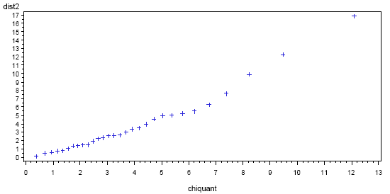
The SAS code used to produce the above graph is as follows:

The data step reads the dataset.

Note: In the upper right-hand corner of the code block you will have the option of copying () the code to your clipboard or downloading () the file to your computer.

data boards;   /*This defines the name of the data set with the name 'boards'.*/
infile "D:\stat505data\boardstiffness.csv" firstobs=2 delimiter=',';   /*This is the path where the contents of the data set are read from.*/
input x1 x2 x3 x4;   /*This is where we provide names for the variables in order of the columns in the data set. If any were categorical (not the case here), we would need to put a '$' character after its name.*/
run;   

proc princomp std out=pcresult;   /*The princomp procedure is primarily used for principal components analysis, which we will see later in this course, but it also provides the Mahalanobis distances we need for producing the QQ plot. The 'out' option specifies the name of a data set used to store results from this procedure.*/
var x1 x2 x3 x4;   /*This specifies that the four variables specified will be used in the princomp calculations.*/
run;   

data mahal;   
set pcresult;   /*This makes the variables in the previously defined data set 'pcresult' available for this new data set 'mahal'.*/
dist2=uss(of prin1-prin4);   /*This calculates the squared Mahalanobis distances from the output generated from the princomp procedure above.*/
run;   

proc print;   /*This prints the specified variable(s) from the data set 'mahal'.*/
var dist2;   /*Only the 'dist2' variable will be printed in this case.*/
run;   

proc sort;   /*This sorts the data set 'mahal' by the variable 'dist2'. We need to do this before constructing the QQ plot in order to match up the squared distances against the correct chi-square quantiles.*/
by dist2;   
run;   

data plotdata;   /*This defines the data set 'plotdata'.*/
set mahal;   /*This makes use of the previously defined data set 'mahal'.*/
prb=(_n_ -.5)/30;   /*This calculates the probabilities to be used in the chi-square quantiles. The _n_ object provides the numbers 1 to 30 (the sample size), and by dividing by the sample size, we effectively divide the range 0 to 1 into 30 points. However, we subtract by 0.5 in order to avoid the limit of 1, since the chi-square quantile at 1 is infinite.*/
chiquant=cinv(prb,4);   
run;   

proc gplot;   /*This produces the QQ plot between the squared distances and the chi-square quantiles computed above.*/
plot dist2*chiquant;   
run;

How to Produce a QQ plot for the Board Stiffness Dataset using Minitab

To construct a QQ plot in Minitab

Open the ‘boardstiffness’ data set in a new worksheet, and calculate the Mahalanobis distances. The steps below assume these distances are stored in the worksheet column ‘Mahal’.
Calc > Calculator
1. In ‘Store result in variable’, enter the name of a new column, such as C7.
2. In the expression window, enter Mahal**2 to square the values of the Mahalanobis distances.
3. Select ‘OK’. The squared Mahalanobis distances should appear in the worksheet under C7.
4. Rename the new column to ‘Mahal2’ for convenience.
Graph > Probability Plot > Simple
1. Highlight and select ‘Mahal2’ to move it to the ‘Graph variables’ window.
2. Choose the ‘Distribution’ button and specify.
  1. Distribution > Gamma (the chi-square is a special case of the gamma)
  2. Shape > 2 for the number of variables divided by 2; in general, this will depend on the number of variables considered for the plot.
  3. Scale > 2
  4. Select ‘OK’.
3. Choose the ‘Scale’ button and check ‘Transpose Y and X’.
4. Select ‘OK’. The QQ plot should appear in the results area.

4.5 - Eigenvalues and Eigenvectors

The next thing that we would like to be able to do is to describe the shape of this ellipse mathematically so that we can understand how the data are distributed in multiple dimensions under a multivariate normal. To do this we first must define the eigenvalues and the eigenvectors of a matrix.

In particular, we will consider the computation of the eigenvalues and eigenvectors of a symmetric matrix \(\textbf{A}\) as shown below:

\(\textbf{A} = \left(\begin{array}{cccc}a_{11} & a_{12} & \dots & a_{1p}\\ a_{21} & a_{22} & \dots & a_{2p}\\ \vdots & \vdots & \ddots & \vdots\\ a_{p1} & a_{p2} & \dots & a_{pp} \end{array}\right)\)

Note: we would call the matrix symmetric if the elements \(a^{ij}\) are equal to \(a^{ji}\) for each i and j.

Usually, \(\textbf{A}\) is taken to be either the variance-covariance matrix \(Σ\), the correlation matrix, or their estimates S and R, respectively.

Eigenvalues and eigenvectors are used for:

Computing prediction and confidence ellipses
Principal Components Analysis (later in the course)
Factor Analysis (also later in this course)

For the present, we will be primarily concerned with eigenvalues and eigenvectors of the variance-covariance matrix.

First of all, let's define what these terms are...

Eigenvalues

If we have a p x p matrix \(\textbf{A}\) we are going to have p eigenvalues, \(\lambda _ { 1 , } \lambda _ { 2 } \dots \lambda _ { p }\). They are obtained by solving the equation given in the expression below:

\(|\textbf{A}-\lambda\textbf{I}|=0\)

On the left-hand side, we have the matrix \(\textbf{A}\) minus \(λ\) times the Identity matrix. When we calculate the determinant of the resulting matrix, we end up with a polynomial of order p. Setting this polynomial equal to zero, and solving for \(λ\) we obtain the desired eigenvalues. In general, we will have p solutions and so there are p eigenvalues, not necessarily all unique.

Eigenvectors

The corresponding eigenvectors \(\mathbf { e } _ { 1 } , \mathbf { e } _ { 2 } , \ldots , \mathbf { e } _ { p }\) are obtained by solving the expression below:

\((\textbf{A}-\lambda_j\textbf{I})\textbf{e}_j = \mathbf{0}\)

Here, we have the difference between the matrix \(\textbf{A}\) minus the \(j^{th}\) eigenvalue times the Identity matrix, this quantity is then multiplied by the \(j^{th}\) eigenvector and set it all equal to zero. This will obtain the eigenvector \(e_{j}\) associated with eigenvalue \(\mu_{j}\).

This does not generally have a unique solution. So, to obtain a unique solution we will often require that \(e_{j}\) transposed \(e_{j}\) is equal to 1. Or, if you like, the sum of the square elements of \(e_{j}\) is equal to 1.

\(\textbf{e}'_j\textbf{e}_j = 1\)

Note! Eigenvectors also correspond to different eigenvalues that are orthogonal. In situations, where two (or more) eigenvalues are equal, corresponding eigenvectors may still be chosen to be orthogonal.

Example 4-3: Consider the 2 x 2 matrix

To illustrate these calculations consider the correlation matrix R as shown below:

\(\textbf{R} = \left(\begin{array}{cc} 1 & \rho \\ \rho & 1 \end{array}\right)\)

Then, using the definition of the eigenvalues, we must calculate the determinant of \(R - λ\) times the Identity matrix.

\(\left|\bf{R} - \lambda\bf{I}\bf\right| = \left|\color{blue}{\begin{pmatrix} 1 & \rho \\ \rho & 1\\ \end{pmatrix}} -\lambda \color{red}{\begin{pmatrix} 1 & 0 \\ 0 & 1\\ \end{pmatrix}}\right|\)

So, \(\textbf{R}\) in the expression above is given in blue, and the Identity matrix follows in red, and \(λ\) here is the eigenvalue that we wish to solve for. Carrying out the math we end up with the matrix with \(1 - λ\) on the diagonal and \(ρ\) on the off-diagonal. Then calculating this determinant we obtain \((1 - λ)^{2} - \rho ^{2}\) squared minus \(ρ^{2}\).

\(\left|\begin{array}{cc}1-\lambda & \rho \\ \rho & 1-\lambda \end{array}\right| = (1-\lambda)^2-\rho^2 = \lambda^2-2\lambda+1-\rho^2\)

Setting this expression equal to zero we end up with the following...

\( \lambda^2-2\lambda+1-\rho^2=0\)

To solve for \(λ\) we use the general result that any solution to the second-order polynomial below:

\(ay^2+by+c = 0\)

is given by the following expression:

\(y = \dfrac{-b\pm \sqrt{b^2-4ac}}{2a}\)

Here, \(a = 1, b = -2\) (the term that precedes \(λ\)) and c is equal to \(1 - ρ^{2}\) Substituting these terms in the equation above, we obtain that \(λ\) must be equal to 1 plus or minus the correlation \(ρ\).

\begin{align} \lambda &= \dfrac{2 \pm \sqrt{2^2-4(1-\rho^2)}}{2}\\ & = 1\pm\sqrt{1-(1-\rho^2)}\\& = 1 \pm \rho \end{align}

Here we will take the following solutions:

\( \begin{array}{ccc}\lambda_1 & = & 1+\rho \\ \lambda_2 & = & 1-\rho \end{array}\)

Next, to obtain the corresponding eigenvectors, we must solve a system of equations below:

\((\textbf{R}-\lambda\textbf{I})\textbf{e} = \mathbf{0}\)

This is the product of \(R - λ\) times I and the eigenvector e set equal to 0. Or in other words, this is translated for this specific problem in the expression below:

\(\left\{\left(\begin{array}{cc}1 & \rho \\ \rho & 1 \end{array}\right)-\lambda\left(\begin{array}{cc}1 &0\\0 & 1 \end{array}\right)\right \}\left(\begin{array}{c} e_1 \\ e_2 \end{array}\right) = \left(\begin{array}{c} 0 \\ 0 \end{array}\right)\)

This simplifies as follows:

\(\left(\begin{array}{cc}1-\lambda & \rho \\ \rho & 1-\lambda \end{array}\right) \left(\begin{array}{c} e_1 \\ e_2 \end{array}\right) = \left(\begin{array}{c} 0 \\ 0 \end{array}\right)\)

Yielding a system of two equations with two unknowns:

\(\begin{array}{lcc}(1-\lambda)e_1 + \rho e_2 & = & 0\\ \rho e_1+(1-\lambda)e_2 & = & 0 \end{array}\)

Note! This does not have a unique solution. If \((e_{1}, e_{2})\) (\(e_{1}\), \(e_{2}\)) is one solution, then a second solution can be obtained by multiplying the first solution by any non-zero constant c, i.e., \((ce_{1}, ce_{2})\). Therefore, we will require the additional condition that the sum of the squared values of \((e_{1}\) and \(e_{2})\) are equal to 1 (ie., \(e^2_1+e^2_2 = 1\))

Consider the first equation:

\((1-\lambda)e_1 + \rho e_2 = 0\)

Solving this equation for \(e_{2}\) and we obtain the following:

\(e_2 = -\dfrac{(1-\lambda)}{\rho}e_1\)

Substituting this into \(e^2_1+e^2_2 = 1\) we get the following:

\(e^2_1 + \dfrac{(1-\lambda)^2}{\rho^2}e^2_1 = 1\)

Recall that \(\lambda = 1 \pm \rho\). In either case we end up finding that \((1-\lambda)^2 = \rho^2\), so that the expression above simplifies to:

\(2e^2_1 = 1\)

Or, in other words:

\(e_1 = \dfrac{1}{\sqrt{2}}\)

Using the expression for \(e_{2}\) which we obtained above,

\(e_2 = -\dfrac{1-\lambda}{\rho}e_1\)

we get

\(e_2 = \dfrac{1}{\sqrt{2}}\) for \(\lambda = 1 + \rho\) and \(e_2 = - \dfrac{1}{\sqrt{2}}\) for \(\lambda = 1-\rho\)

Therefore, the two eigenvectors are given by the two vectors as shown below:

\(\left(\begin{array}{c}\frac{1}{\sqrt{2}}\\ \frac{1}{\sqrt{2}} \end{array}\right)\) for \(\lambda_1 = 1+ \rho\) and \(\left(\begin{array}{c}\frac{1}{\sqrt{2}}\\ -\frac{1}{\sqrt{2}} \end{array}\right)\) for \(\lambda_2 = 1- \rho\)

Some properties of the eigenvalues of the variance-covariance matrix are to be considered at this point. Suppose that \(\mu_{1}\) through \(\mu_{p}\) are the eigenvalues of the variance-covariance matrix \(Σ\). By definition, the total variation is given by the sum of the variances. It turns out that this is also equal to the sum of the eigenvalues of the variance-covariance matrix. Thus, the total variation is:

\(\sum_{j=1}^{p}s^2_j = s^2_1 + s^2_2 +\dots + s^2_p = \lambda_1 + \lambda_2 + \dots + \lambda_p = \sum_{j=1}^{p}\lambda_j\)

The generalized variance is equal to the product of the eigenvalues:

\(|\Sigma| = \prod_{j=1}^{p}\lambda_j = \lambda_1 \times \lambda_2 \times \dots \times \lambda_p\)

4.6 - Geometry of the Multivariate Normal Distribution

The geometry of the multivariate normal distribution can be investigated by considering the orientation, and shape of the prediction ellipse as depicted in the following diagram:

plot

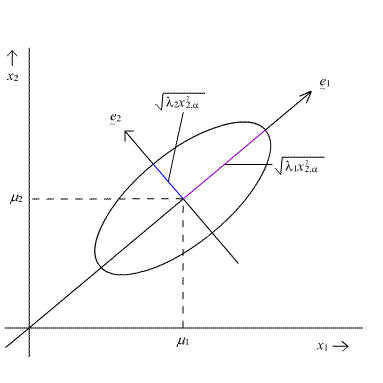
The \((1 - α) \times 100%\) prediction ellipse above is centered on the population means \(\mu_{1}\) and \(\mu_{2}\).

The ellipse has axes pointing in the directions of the eigenvectors \(e _ { 1 } , e _ { 2 } , \dots , e _ { p } \). Here, in this diagram for the bivariate normal, the longest axis of the ellipse points in the direction of the first eigenvector \(e_{1}\) and the shorter axis is perpendicular to the first, pointing in the direction of the second eigenvector \(e_{2}\).

The corresponding half-lengths of the axes are obtained by the following expression:

\(l_j = \sqrt{\lambda_j\chi^2_{p,\alpha}}\)

The plot above captures the lengths of these axes within the ellipse.

The volume (area) of the hyper-ellipse is equal to:

\(\dfrac{2\pi^{p/2}}{p\Gamma\left(\frac{p}{2}\right)}(\chi^2_{p,\alpha})^{p/2}|\Sigma|^{1/2}\)

Note! This is a function of the square root of the generalized variance (given by the square root of the determinant of the variance-covariance matrix). Thus, the volume (area) of the prediction ellipse is proportional to the square root of the generalized variance.

In this expression for the volume (area) of the hyper-ellipse, \(Γ(x)\) is the gamma function. To compute the gamma function, consider the two special cases:

Case I: p is even

\(\Gamma\left(\frac{p}{2}\right) = \left(\frac{p}{2}-1\right)!\)

Case II: p is odd

\(\Gamma\left(\frac{p}{2}\right) = \dfrac{1 \times 3 \times 5 \times \dots \times (p-2) \times \sqrt{\pi}}{2^{(p-1)/2}}\)

We shall illustrate the shape of the multivariate normal distribution using the Wechsler Adult Intelligence Scale data.

4.7 - Example: Wechsler Adult Intelligence Scale

Example 4-4: Wechsler Adult Intelligence Scale

Here we have data on n = 37 subjects taking the Wechsler Adult Intelligence Test. This test is broken up into four different components:

Information (Info)
Similarities (Sim)
Arithmetic (Arith)
Picture Completion (Pic)

The data are stored in five different columns. The first column is the ID number of the subjects, followed by the four component tasks in the remaining four columns.

Download the txt file: wechsler.csv

Using Technology

Example
Example

These data may be analyzed using the SAS program shown below.

Download the SAS file: wechsler.sas

Note: In the upper right-hand corner of the code block you will have the option of copying () the code to your clipboard or downloading () the file to your computer.

options ls=78;
title "Eigenvalues and Eigenvectors - Wechsler Data";

 /* The first two lines define the name of the data set with the name 'wechsler'
  * and specify the path where the contents of the data set are read from.
  * Since we have a header row, the first observation begins on the 2nd row,
  * and the delimiter option is needed because columns are separated by commas.
  * The input statement is where we provide names for the variables in order 
  * of the columns in the data set. If any were categorical (not the case here), 
  * we would need to put a '$' character after its name.
  */

data wechsler;
  infile "D:\Statistics\STAT 505\data\wechsler.csv" firstobs=2 delimiter=',';
  input id info sim arith pict;
  run;

 /* This prints the specified variable(s) from the data set 'wechsler'. 
  * Since no variables are specified, all are printed.
  */

proc print data=wechsler;
  run;

 /* The princomp procedure calculates the eigenvalues and eigenvectors 
  * for the variables specified in the var statement. The default is 
  * to operate on the correlation matrix of the data, but the 'cov' option 
  * indicates to use the covariance matrix instead.
  */

proc princomp data=wechsler cov;
  var info sim arith pict;
  run;

Walk through the procedures of the program by clicking on the "Explore the code" button. Just as in previous lessons, marking up a printout of the SAS program is also a good strategy for learning how this program is put together.

The SAS output, (download below), gives the results of the data analyses. Because the SAS output is usually a relatively long document, printing these pages of output out and marking them with notes is highly recommended if not required!!

Download the SAS output here: wechsler.lst

Produce the Covariance Matrix for the Wechsler Adult Intelligence Test Data

To find the sample covariance matrix of a multivariate data set:

Stat > Basic Statistics > Covariance
1. Highlight and select the names of all the variables of interest to move them into the window on the right.
2. Check the box for ‘Store matrix’.
3. Select ‘OK’. No results are displayed at this point.
Data > Display Data
1. Highlight and select M1 and choose ‘Select’ to move it into the window on the right.
2. Select ‘OK’ to display the sample covariance matrix.

Analysis

We obtain the following sample means.

Variable	Mean
Information	12.568
Similarities	9.568
Arithmetic	11.486
Picture Completion	7.973

Variance-Covariance Matrix

\(\textbf{S} = \left(\begin{array}{rrrr}11.474 & 9.086 & 6.383 & 2.071\\ 9.086 & 12.086 & 5.938 & 0.544\\ 6.383 & 5.938 & 11.090 & 1.791\\ 2.071 & 0.544 & 1.791 & 3.694 \end{array}\right)\)

Here, for example, the variance for Information was 11.474. For Similarities, it was 12.086. The covariance between Similarities and Information is 9.086. The total variance, which is the sum of the variances comes out to be 38.344, approximately.

The eigenvalues are given below:

\(\lambda_1 = 26.245\), \(\lambda_2 = 6.255\), \(\lambda_3 = 3.932\), \(\lambda_4 = 1.912\)

and finally, at the bottom of the table, we have the corresponding eigenvectors. They have been listed here below:

\(\mathbf{e_1}=\left(\begin{array}{r}0.606\\0.605\\0.505\\0.110 \end{array}\right)\), \(\mathbf{e_2}=\left(\begin{array}{r}-0.218\\-0.496\\0.795\\0.274 \end{array}\right)\), \(\mathbf{e_3}=\left(\begin{array}{r}0.461\\-0.320\\-0.335\\0.757 \end{array}\right)\), \(\mathbf{e_4}=\left(\begin{array}{r}-0.611\\0.535\\-0.035\\0.582 \end{array}\right)\)

For example, the eigenvectors corresponding to the eigenvalue 26.245, those elements are 0.606, 0.605, 0.505, and 0.110.

Now, let's consider the shape of the 95% prediction ellipse formed by the multivariate normal distribution whose variance-covariance matrix is equal to the sample variance-covariance matrix we just obtained.

Recall the formula for the half-lengths of the axis of this ellipse. This is equal to the square root of the eigenvalue times the critical value from a chi-square table. In this case, we need the chi-square with four degrees of freedom because we have four variables. For a 95% prediction ellipse, the chi-square with four degrees of freedom is equal to 9.49.

For looking at the first and longest axis of a 95% prediction ellipse, we substitute 26.245 for the largest eigenvalue, multiplied by 9.49, and take the square root. We end up with a 95% prediction ellipse with a half-length of 15.782 as shown below:

\begin{align} l_1 &= \sqrt{\lambda_1\chi^2_{4,0.05}}\\ &= \sqrt{26.245 \times 9.49}\\ &= 15.782 \end{align}

The direction of the axis is given by the first eigenvector. Looking at this first eigenvector we can see large positive elements corresponding to the first three variables. In other words, large elements for Information, Similarities, and Arithmetic. This suggests that this particular axis points in the direction specified by \(e_{1}\); that is, increasing values of Information, Similarities, and Arithmetic.

The half-length of the second longest axis can be obtained by substituting 6.255 for the second eigenvalue, multiplying this by 9.49, and taking the square root. We obtain a half-length of about 7.7 or about half the length of the first axis.

\begin{align} l_2 &= \sqrt{\lambda_2\chi^2_{4,0.05}}\\ &= \sqrt{6.255 \times 9.49}\\ &= 7.705 \end{align}

So, if you were to picture this particular ellipse you would see that the second axis is about half the length of the first and longest axis.

Looking at the corresponding eigenvector, \(e_{2}\), we can see that this particular axis is pointed in the direction of points in the direction of increasing values for the third value, or Arithmetic and decreasing value for Similarities, the second variable.

Similar calculations can then be carried out for the third-longest axis of the ellipse as shown below:

\begin{align} l_3 &= \sqrt{\lambda_1\chi^2_{4,0.05}}\\ &= \sqrt{3.931 \times 9.49}\\ &= 6.108 \end{align}

This third axis has a half-length of 6.108, which is not much shorter or smaller than the second axis. It points in the direction of \(e_{3}\)that is, increasing values of Picture Completion and Information, and decreasing values of Similarities and Arithmetic.

The shortest axis has a half-length of about 4.260 as shown below:

\begin{align} l_4 &= \sqrt{\lambda_4\chi^2_{4,0.05}}\\ &= \sqrt{1.912 \times 9.49}\\ &= 4.260 \end{align}

It points in the direction of \(e_{4}\) that is, increasing values of Similarities and Picture Completion, and decreasing values of Information.

The overall shape of the ellipse can be obtained by comparing the lengths of the various axis. What we have here is basically an ellipse that is the shape of a slightly squashed football.

We can also obtain the volume of the hyper-ellipse using the formula that was given earlier. Again, our critical value from the chi-square, if we are looking at a 95% prediction ellipse, with four degrees of freedom is given at 9.49. Substituting into our expression we have the product of the eigenvalues in the square root. The gamma function is evaluated at 2, and a gamma of 2 is simply equal to 1. Carrying out the math we end up with a volume of 15,613.132 as shown below:

\begin{align} \frac{2\pi^{p/2}}{p\Gamma\left(\frac{p}{2}\right)}(\chi^2_{p,\alpha})^{p/2}|\Sigma|^{1/2} &= \frac{2\pi^{p/2}}{p\Gamma\left(\frac{p}{2}\right)}(\chi^2_{p,\alpha})^{p/2}\sqrt{\prod_{j=1}^{p}\lambda_j} \\[10pt] &= \frac{2\pi^2}{4\Gamma(2)}(9.49)^2\sqrt{26.245 \times 6.255 \times 3.932 \times 1.912}\\[10pt] &= 444.429 \sqrt{1234.17086}\\[10pt] &= 15613.132\end{align}

4.8 - Special Cases: p = 2

To further understand the shape of the multivariate normal distribution, let's return to the special case where we have p = 2 variables.

If \(ρ = 0\), there is zero correlation, and the eigenvalues turn out to be equal to the variances of the two variables. So, for example, the first eigenvalue would be equal to \(\sigma^2_1\) and the second eigenvalue would be equal to \(\sigma^2_2\) as shown below:

\(\lambda_1 = \sigma^2_1\) and \(\lambda_2 = \sigma^2_2\)

the corresponding eigenvectors will have elements 1 and 0 for the first eigenvalue and 0 and 1 for the second eigenvalue.

\(\mathbf{e}_1 = \left(\begin{array}{c} 1\\ 0\end{array}\right)\), \(\mathbf{e}_2 = \left(\begin{array}{c} 0\\ 1\end{array}\right)\)

So, the axis of the ellipse, in this case, is parallel to the coordinate axis.

If there is zero correlation, and the variances are equal so that \(\sigma^2_1\) = \(\sigma^2_2\), then the eigenvalues will be equal to one another, and instead of an ellipse we will get a circle. In this special case, we have a so-called circular normal distribution.

SAS plot

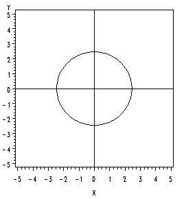
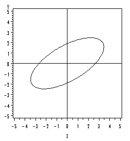
If the correlation is greater than zero, then the longer axis of the ellipse will have a positive slope.

SAS plot

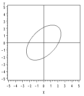
Conversely, if the correlation is less than zero, then the longer axis of the ellipse will have a negative slope.

As the correlation approaches plus or minus 1, the larger eigenvalue will approach the sum of the two variances, and the smaller eigenvalue will approach zero:

\(\lambda_1 \rightarrow \sigma^2_1 +\sigma^2_2\) and \(\lambda_2 \rightarrow 0\)

So, what is going to happen in this case is that the ellipse becomes more and more elongated as the correlation approaches one.

Using Technology

Example
Example

The SAS program below can be used to plot the 95% confidence ellipse corresponding to any specified variance-covariance matrix.

Download the SAS program here: ellplot.sas

Note: In the upper right-hand corner of the code block you will have the option of copying () the code to your clipboard or downloading () the file to your computer.

options ls=78;   
title "95% prediction ellipse";   

data a;   /*This data set defines the polar coordinates for plotting the prediction ellipse as a function of the angle theta. It stores the results in variables 'u' and 'v' that will be used below.*/
  pi=2.d0*arsin(1);   
  do i=0 to 200;   
    theta=pi*i/100;   
    u=cos(theta);   
    v=sin(theta);   
    output;   
  end;   
  run;   

proc iml;   /*The iml procedure allows for many general calculations to be made. In this case*/
  create b var{x y};   /*This defines a data set 'b' with two variables 'x' and 'y' that will be used in the calculations below.*/
  start ellipse;   /*This defines a SAS module named 'ellipse' that can be called to calculate the xy coordinates for ploting the prediction ellipse. The lines of code below are executed when 'ellipse' is called.*/
    mu={0,   /*This specifies the value of the bivariate mean vector (0, 0). This will be the center of the prediction ellipse.*/
        0};   
    sigma={1.0000 0.5000,   /*This specifies the values of the covariance matrix, which must be symmetric.*/
           0.5000 2.0000};   
    lambda=eigval(sigma);   /*The statements below calculate the xy coordinates for plotting the ellipse from the polar coordinates that are provided above.*/
    e=eigvec(sigma);   
    d=diag(sqrt(lambda));   
    z=z*d*e`*sqrt(5.99);   
    do i=1 to nrow(z);   
      x=z[i,1];   
      y=z[i,2];   
      append;   
    end;   
  finish;   /*This ends the module definition.*/
  use a;   /*This makes the polar coordinates defined in the data set 'a' available.*/
  read all var{u v} into z;   /*The polar coordinates are assigned to the vector z, which is used in the ellipse module.*/
  run ellipse;   /*This calls the ellipse module, which runs and populates the data set 'b' with the xy coordinates that will be used for plotting the prediction ellipse.*/

proc gplot;   /*This plots the prediction ellipse from the coordinates in the data set 'b'.*/
  axis1 order=-5 to 5 length=3 in;   /*The axis statements set the limits of the plotting region.*/
  axis2 order=-5 to 5 length=3 in;   
  plot y*x / vaxis=axis1 haxis=axis2 vref=0 href=0;   /*These options specify the variables for plotting, which to put on which axis, and the vertical and horizontal reference lines.*/
  symbol v=none l=1 i=join color=black;   /*This option specifies that the points are to be joined in a continuous curve in black.*/
  run;

The bivariate confidence interval for this example cannot be generated using Minitab.

4.9 Summary

In this lesson we learned about:

The probability density function for the multivariate normal distribution
The definition of a prediction ellipse
How the shape of the multivariate normal distribution depends on the variances and covariances
The definitions of eigenvalues and eigenvectors of a matrix, and how they may be computed
How to determine the shape of the multivariate normal distribution from the eigenvalues and eigenvectors of the variance-covariance matrix

^[1]	Link
↥	Has Tooltip/Popover
	Toggleable Visibility

Lesson 4: Multivariate Normal Distribution

Overview

Objectives

4.1 - Comparing Distribution Types

Univariate Normal Distributions

Multivariate Normal Distributions

Other Useful Results for the Multivariate Normal

Example 4-1 - Linear Combination of the Cholesterol Measurements

4.2 - Bivariate Normal Distribution

Bivariate Normal Distribution

Using Technology

How to Use Minitab to Create Plots of the Bivariate Distribution.

To plot a bivariate normal density for a given correlation value:

4.3 - Exponent of Multivariate Normal Distribution

Useful facts about the Exponent Component: \( (\textbf{x}-\mathbf{\mu})'\Sigma^{-1}(\textbf{x}-\mathbf{\mu})\)

Using Technology

Calculating Mahalanobis Distance With SAS

Example - Calculating and Printing Mahalonobis Distances in SAS

To calculate the Mahalanobis distances in Minitab:

4.4 - Multivariate Normality and Outliers

Q-Q Plot for Evaluating Multivariate Normality and Outliers

Determining the Quantiles

Example 4-2: Q-Q Plot for Board Stiffness Data

How to Produce a QQ plot for the Board Stiffness Dataset using Minitab

To construct a QQ plot in Minitab

4.5 - Eigenvalues and Eigenvectors

Example 4-3: Consider the 2 x 2 matrix

4.6 - Geometry of the Multivariate Normal Distribution

Case I: p is even

Case II: p is odd

4.7 - Example: Wechsler Adult Intelligence Scale

Example 4-4: Wechsler Adult Intelligence Scale

Produce the Covariance Matrix for the Wechsler Adult Intelligence Test Data

Analysis

Variance-Covariance Matrix

4.8 - Special Cases: p = 2

Using Technology

4.9 Summary