1.5 - Additional Measures of Dispersion
1.5 - Additional Measures of DispersionOverall Measures of Dispersion
Sometimes it is also useful to have an overall measure of dispersion in the data. In this measure, it would be good to include all of the variables simultaneously, rather than one at a time. In the past, we looked at the individual variables and their variances to measure the individual variances. Here we are going to look at measures of dispersion of all variables together, particularly we are going to look at such measures that look at the total variation.
The variance \(\sigma _{j}^{2}\) measures the dispersion of an individual variable Xj. The following two are used to measure the dispersion of all variables together.
- Total Variation
- Generalized Variance
To understand total variation we first must find the trace of a square matrix. A square matrix is a matrix that has an equal number of columns and rows. Important examples of square matrices include the variance-covariance and correlation matrices.
- Trace of an n x n Matrix
- The trace of an n x n matrix \(\mathbf{A}\) is
- \(trace(\textbf{A}) = \sum_{i=1}^{n}a_{ii}\)
For instance, in a 10 x 10 matrix, the trace is the sum of the diagonal elements.
- Total Variation of a Random Vector, \(\mathbf{X}\)
-
The total variation, therefore, of a random vector \(\mathbf{X}\) is simply the trace of the population variance-covariance matrix.
\(trace (\Sigma) = \sigma^2_1 + \sigma^2_2 +\dots \sigma^2_p\)
Thus, the total variation is equal to the sum of the population variances.
The total variation can be estimated by:
\(trace(S) = s^2_1+s^2_2+\dots +s^2_p\)
The total variation is of interest for principal components analysis and factor analysis and we will look at these concepts later in this course.
Example 1-6: Woman's Health Survey (Variance)
Let us use the data from the USDA women’s health survey again to illustrate this. We have taken the variances for each of the variables from the software output and have placed them in the table below.
| Variable | Variance |
|---|---|
| Calcium | 157829.4 |
| Iron | 35.8 |
| Protein | 934.9 |
| Vitamin A | 2668452.4 |
| Vitamin C | 5416.3 |
| Total | 2832668.8 |
The total variation for the nutrient intake data is determined by simply adding up all of the variances for each of the individual variables. The total variation equals 2,832,668.8. This is a very large number.
Interpreting Correlation
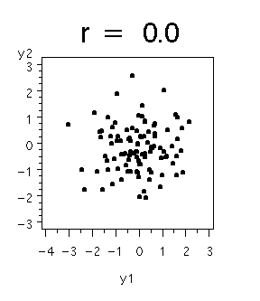
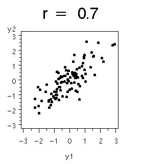
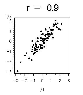
These plots show simulated data for pairs of variables with different levels of correlation. In each case, the variances for both variables are equal to 1, so that the total variation is 2.
When the correlation r = 0, then we see a shotgun-blast pattern of points, widely dispersed over the entire range of the plot.

Increasing the correlation to r = 0.7, we see an oval-shaped pattern. Note that the points are not as widely dispersed.

Increasing the correlation to r = 0.9, we see that the points fall along a 45-degree line, and are even less dispersed.

Thus, the dispersion of points decreases with increasing correlation. But, in all cases, the total variation is the same. The total variation does not take into account the correlation between the two variables.
Fixing the variances, the scatter of the data will tend to decrease as \(| r | \rightarrow 1\).
The Determinant
To take into account the correlations among pairs of variables an alternative measure of overall variance is suggested. This measure takes a large value when the various variables show very little correlation among themselves. In contrast, this measure takes a small value if the variables show a very strong correlation among themselves, either positive or negative. This particular measure of dispersion is the generalized variance. In order to define the generalized variance, we first define the determinant of the matrix.
We will start simple with a 2 x 2 matrix and then we will move on to more general definitions for larger matrices.
Let us consider the determinant of a 2 x 2 matrix \(\mathbf{B}\) as shown below. Here we can see that it is the product of the two diagonal elements minus the product of the off-diagonal elements.
\(|\textbf{B}| =\left|\begin{array}{cc}b_{11} & b_{12}\\ b_{21} & b_{22}\end{array}\right| = b_{11}b_{22}-b_{12}b_{21}\)
Here is an example of a simple matrix that has the elements 5, 1, 2, and 4. You will get the determinant 18. The product of the diagonal 5 x 4 subtracting the elements of the off-diagonal 1 x 2 yields an answer of 18:
\(\left|\begin{array}{cc}5 & 1\\2 & 4\end{array}\right| = 5 \times 4 - 1\times 2= 20-2 =18\)
- Determinant of a General \(p\ x\ p\) Matrix \(\mathbf{B}\)
-
More generally the determinant of a general p x p matrix \(\mathbf{B}\) is given by the expression shown below:
- \(|\textbf{B}| = \sum_{j=1}^{p}(-1)^{j+1}b_{1j}|B_{1j}|\)
The expression involves the sum over all of the first row of \(\mathbf{B}\). Note that these elements are noted by \(b_{1j}\). These are pre-multiplied by -1 raised to the \([j + 1]^{th}\) power, so basically we are going to have alternating plus and minus signs in our sum. The matrix \(B1_j\) is obtained by deleting row 1 and column j from the matrix \(\mathbf{B}\).
By definition, the generalized variance of a random vector \(\mathbf{X}\) is equal to \(|\sum|\), the determinant of the variance/covariance matrix. The generalized variance can be estimated by calculating \(|S|\), the determinant of the sample variance/covariance matrix.