12.10 - Factor Rotations
12.10 - Factor RotationsFrom our experience with the Places Rated data, it does not look like the factor model works well. There is no guarantee that any model will fit the data well.
The first motivation of factor analysis was to try to discern some underlying factors describing the data. The Maximum Likelihood Method failed to find such a model to describe the Places Rated data. The second motivation is still valid, which is to try to obtain a better interpretation of the data. In order to do this, let's take a look at the factor loadings obtained before from the principal component method.
| Factor | |||
|---|---|---|---|
| Variable | 1 | 2 | 3 |
| Climate | 0.286 | 0.076 | 0.841 |
| Housing | 0.698 | 0.153 | 0.084 |
| Health | 0.744 | -0.410 | -0.020 |
| Crime | 0.471 | 0.522 | 0.135 |
| Transportation | 0.681 | -0.156 | -0.148 |
| Education | 0.498 | -0.498 | -0.253 |
| Arts | 0.861 | -0.115 | 0.011 |
| Recreation | 0.642 | 0.322 | 0.044 |
| Economics | 0.298 | 0.595 | -0.533 |
The problem with this analysis is that some of the variables are highlighted in more than one column. For instance, Education appears significant to Factor 1 AND Factor 2. The same is true for Economics in both Factors 2 AND 3. This does not provide a very clean, simple interpretation of the data. Ideally, each variable would appear as a significant contributor in one column.
In fact, the above table may indicate contradictory results. Looking at some of the observations, it is conceivable that we will find an observation that takes a high value on both Factors 1 and 2. If this occurs, a high value for Factor 1 suggests that the community has quality education, whereas a high value for Factor 2 suggests the opposite, that the community has poor education.
Factor rotation is motivated by the fact that factor models are not unique. Recall that the factor model for the data vector, \(\mathbf{X = \boldsymbol{\mu} + LF + \boldsymbol{\epsilon}}\), is a function of the mean \(\boldsymbol{\mu}\), plus a matrix of factor loadings times a vector of common factors, plus a vector of specific factors.
Moreover, we should note that this is equivalent to a rotated factor model, \(\mathbf{X = \boldsymbol{\mu} + L^*F^* + \boldsymbol{\epsilon}}\), where we have set \(\mathbf{L^* = LT}\) and \(\mathbf{f^* = T'f}\) for some orthogonal matrix \(\mathbf{T}\) where \(\mathbf{T'T = TT' = I}\). Note that there are an infinite number of possible orthogonal matrices, each corresponding to a particular factor rotation.
We plan to find an appropriate rotation, defined through an orthogonal matrix \(\mathbf{T}\), that yields the most easily interpretable factors.
To understand this, consider a scatter plot of factor loadings. The orthogonal matrix \(\mathbf{T}\) rotates the axes of this plot. We wish to find a rotation such that each of the p variables has a high loading on only one factor.
We will return to the program below to obtain a plot. In looking at the program, there are a number of options (marked in blue under proc factor) that we did not yet explain.
Download the SAS program here: places2.sas
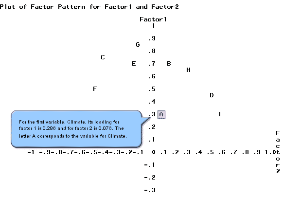
One of the options above is labeled 'preplot'. We will use this to plot the values for factor 1 against factor 2.
In the output these values are plotted, the loadings for factor 1 on the y-axis, and the loadings for factor 2 on the x-axis.

Similarly, the second variable, labeled with the letter B, has a factor 1 loading of about 0.7 and a factor 2 loading of about 0.15. Each letter on the plot corresponds to a single variable. SAS provides plots of the other combinations of factors, factor 1 against factor 3 as well as factor 2 against factor 3.
Three factors appear in this model so we might consider a three-dimensional plot of all three factors together.
Obtaining a scree plot and loading plot
To perform factor analysis with scree and loading plots:
- Open the ‘places_tf.csv’ data set in a new worksheet.
- Transform variables. This step is optional but used in the steps below.
- Calc > Calculator
- Highlight and select ‘climate’ to move it to the Store result window.
- In the Expression window, enter LOGTEN( 'climate') to apply the (base 10) log transformation to the climate variable.
- Choose OK. The transformed values replace the originals in the worksheet under ‘climate’.
- Repeat sub-steps 1) through 4) above for all variables housing through econ.
- Stat > Multivariate > Factor Analysis
- Highlight and select climate through econ to move all 9 variables to the Variables window.
- Choose 3 for the number of factors to extract.
- Choose Principal Components for the Method of Extraction.
- Under Graphs, select Scree plot and Loading plot for first two factors.
- Choose OK and OK again. The numeric results are shown in the results area, along with both the scree plot and the loading plot.
The selection of the orthogonal matrixes \(\mathbf{T}\) corresponds to our rotation of these axes. Think about rotating the axis of the center. Each rotation will correspond to an orthogonal matrix \(\mathbf{T}\). We want to rotate the axes to obtain a cleaner interpretation of the data. We would really like to define new coordinate systems so that when we rotate everything, the points fall close to the vertices (endpoints) of the new axes.
If we were only looking at two factors, then we would like to find each of the plotted points at the four tips (corresponding to all four directions) of the rotated axes. This is what rotation is about, taking the factor pattern plot and rotating the axes in such a way that the points fall close to the axes.