12.11 - Varimax Rotation
12.11 - Varimax Rotation- Varimax Rotation
- Varimax rotation is the most common. It involves scaling the loadings by dividing them by the corresponding communality as shown below:
- \(\tilde{l}^*_{ij}= \hat{l}^*_{ij}/\hat{h}_i\)
- Varimax rotation finds the rotation that maximizes this quantity. The Varimax procedure, as defined below, selects the rotation in order to maximize
- \(V = \frac{1}{p}\sum\limits_{j=1}^{m}\left\{\sum\limits_{i=1}^{p}(\tilde{l}^*_{ij})^4 - \frac{1}{p}\left(\sum\limits_{i=1}^{p}(\tilde{l}^*_{ij})^2 \right)^2 \right\}\)
This is the sample variances of the standardized loadings for each factor summed over the m factors.
Returning to the options of the factoring procedure (marked in blue):
"rotate," asks for factor rotation and we specified the Varimax rotation of our factor loadings.
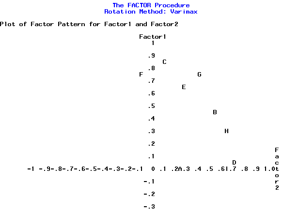
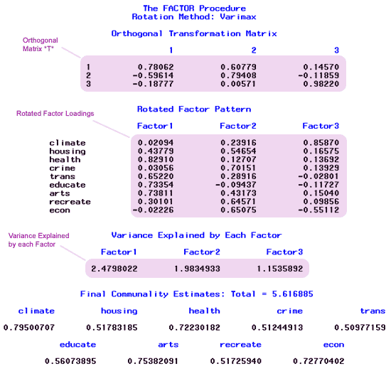
"plot," asks for the same kind of plot that we just looked at for the rotated factors. The result of our rotation is a new factor pattern given below (page 11 of SAS output):

Here is a copy of page 10 from the SAS output:

At the top of page 10 of the output, above, we have our orthogonal matrix T.
Using Varimax Rotation
To perform factor analysis with varimax rotation:
- Open the ‘places_tf.csv’ data set in a new worksheet.
- Transform variables. This step is optional but used in the steps below.
- Calc > Calculator
- Highlight and select ‘climate’ to move it to the Store result window.
- In the Expression window, enter LOGTEN( 'climate') to apply the (base 10) log transformation to the climate variable.
- Choose OK. The transformed values replace the originals in the worksheet under ‘climate’.
- Repeat sub-steps 1) through 4) above for all variables housing through econ.
- Stat > Multivariate > Factor Analysis
- Highlight and select climate through econ to move all 9 variables to the Variables window.
- Choose 3 for the number of factors to extract.
- Choose Principal Components for the Method of Extraction.
- Choose Varimax for the Type of Rotation.
- Under Graphs, select Loading plot for the first two factors.
- Choose OK and OK again. The numeric results are shown in the results area, along with the loading plot.
The values of the rotated factor loadings are:
| Factor | |||
|---|---|---|---|
| Variable | 1 | 2 | 3 |
| Climate | 0.021 | 0.239 | 0.859 |
| Housing | 0.438 | 0.547 | 0.166 |
| Health | 0.829 | 0.127 | 0.137 |
| Crime | 0.031 | 0.702 | 0.139 |
| Transportation | 0.652 | 0.289 | -0.028 |
| Education | 0.734 | -0.094 | -0.117 |
| Arts | 0.738 | 0.432 | 0.150 |
| Recreation | 0.301 | 0.656 | 0.099 |
| Economics | -0.022 | 0.651 | -0.551 |
Let us now interpret the data based on the rotation. We highlighted the values that are large in magnitude and make the following interpretation.
- Factor 1: primarily a measure of Health, but also increases with increasing scores for Transportation, Education, and the Arts.
- Factor 2: primarily a measure of Crime, Recreation, the Economy, and Housing.
- Factor 3: primarily a measure of Climate alone.
This is just the pattern that exists in the data and no causal inferences should be made from this interpretation. It does not tell us why this pattern exists. It could very well be that there are other essential factors that are not seen at work here.
Let us look at the amount of variation explained by our factors under the rotated model and compare it to the original model. Consider the variance explained by each factor under the original analysis and the rotated factors:
| Analysis | ||
|---|---|---|
| Factor | Original | Rotated |
| 1 | 3.2978 | 2.4798 |
| 2 | 1.2136 | 1.9835 |
| 3 | 1.1055 | 1.1536 |
| Total | 5.6169 | 5.6169 |
The total amount of variation explained by the 3 factors remains the same. Rotations, among a fixed number of factors, do not change how much of the variation is explained by the model. The fit is equally good regardless of what rotation is used.
However, notice what happened to the first factor. We see a fairly large decrease in the amount of variation explained by the first factor. We obtained a cleaner interpretation of the data but it costs us something somewhere. The cost is that the variation explained by the first factor is distributed among the latter two factors, in this case mostly to the second factor.
The total amount of variation explained by the rotated factor model is the same, but the contributions are not the same from the individual factors. We gain a cleaner interpretation, but the first factor does not explain as much of the variation. However, this would not be considered a particularly large cost if we are still interested in these three factors.
Rotation cleans up the interpretation. Ideally, we should find that the numbers in each column are either far away from zero or close to zero. Numbers close to +1 or -1 or 0 in each column give the ideal or cleanest interpretation. If a rotation can achieve this goal, then that is wonderful. However, observed data are seldom this cooperative!
Nevertheless, recall that the objective is data interpretation. The success of the analysis can be judged by how well it helps you to make sense of your data If the result gives you some insight as to the pattern of variability in the data, even without being perfect, then the analysis was successful.