7.2.2 - Upon Which Variable do the Swiss Banknotes Differ? -- Two Sample Mean Problem

When the hypothesis of equality of two independent population means is rejected, one would like to know on account of which variable the hypothesis is rejected. To assess that, we go back to the example of Swiss Banknotes.

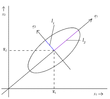
To assess which variable these notes differ on we will consider the \(( 1 - \alpha ) \times 100 \%\) Confidence Ellipse for the difference in the population mean vectors for the two populations of banknotes, \(\boldsymbol{\mu_{1}}\) - \(\boldsymbol{\mu_{2}}\). This ellipse is given by the set of \(\boldsymbol{\mu_{1}}\) satisfying the expression:

\(\mathbf{(\bar{x}_1-\bar{x}_2-(\pmb{\mu}_1-\pmb{\mu}_2))}'\left\{\mathbf{S}_p \left(\dfrac{1}{n_1}+\dfrac{1}{n_2}\right) \right\}^{-1}\mathbf{(\bar{x}_1-\bar{x}_2-(\pmb{\mu}_1-\pmb{\mu}_2))} \le \dfrac{p(n_1+n_2-2)}{n_1+n_2-p-1}F_{p,n_1+n_2-p-1,\alpha}\)

To understand the geometry of this ellipse, let

\(\lambda_1, \lambda_2, \dots, \lambda_p\)

denote the eigenvalues of the pooled variance-covariance matrix \(S_{p}\), and let

\(\mathbf{e}_{1}\), \(\mathbf{e}_{2}\), ..., \(\mathbf{e}_{p}\)

denote the corresponding eigenvectors. Then the \(k^{th}\) axis of this p dimensional ellipse points in the direction specified by the \(k^{th}\) eigenvector, \(\mathbf{e}_{k}\) And, it has a half-length given by the expression below:

\[l_k = \sqrt{\lambda_k\frac{p(n_1+n_2-2)}{n_1+n_2-p-1}\left(\frac{1}{n_1}+\frac{1}{n_2}\right)F_{p,n_1+n_2-p-1,\alpha}}\]

Note, again, that this is a function of the number of variables, p, the sample sizes \(n_{1}\) and \(n_{2}\), and the critical value from the F-table.

The \(( 1 - \alpha ) \times 100 \%\) confidence ellipse yields simultaneous \(( 1 - \alpha ) \times 100 \%\) confidence intervals for all linear combinations of the form given in the expression below:

\(c_1(\mu_{11}-\mu_{21})+c_2(\mu_{12}-\mu_{22})+\dots+c_p(\mu_{1p}-\mu_{2p}) = \sum_{k=1}^{p}c_k(\mu_{1k}-\mu_{2k}) = \mathbf{c'(\mu_1-\mu_k)}\)

So, these are all linear combinations of the differences in the sample means between the two populations where we are taking linear combinations across variables. These simultaneous confidence intervals are given by the expression below:

\(\sum_{k=1}^{p}c_k(\bar{x}_{1k}-\bar{x}_{2k}) \pm \sqrt{\dfrac{p(n_1+n_2-2)}{n_1+n_2-p-1}F_{p,n_1+n_2-p-1,\alpha}}\sqrt{\left(\dfrac{1}{n_1}+\dfrac{1}{n_2}\right) \sum_{k=1}^{p}\sum_{l=1}^{p}c_kc_ls^{(p)}_{kl}}\)

Here, the terms \(s^{(p)}_{kl}\) denote the pooled covariances between variables k and l.

Interpretation

The interpretation of these confidence intervals is the same as that for the one sample of Hotelling's T-square. Here, we are \(( 1 - \alpha ) \times 100 \%\) confident that all of these intervals cover their respective linear combinations of the differences between the means of the two populations. In particular, we are also \(( 1 - \alpha ) \times 100 \%\) confident that all of the intervals of the individual variables also cover their respective differences between the population means. For the individual variables, if we are looking at, say, the \(k^{th}\) individual variable, then we have the difference between the sample means for that variable, k, plus or minus the same radical term that we had in the expression previously, times the standard error of that difference between the sample means for the \(k^{th}\) variable. The latter involves the inverses of the sample sizes and the pooled variance for variable k.

\(\bar{x}_{1k}-\bar{x}_{2k} \pm \sqrt{\dfrac{p(n_1+n_2-2)}{n_1+n_2-p-1}F_{p,n_1+n_2-p-1,\alpha}}\sqrt{\left(\dfrac{1}{n_1}+\dfrac{1}{n_2}\right) s^2_k}\)

So, here, \(s^2_k\) is the pooled variance for variable k. These intervals are called simultaneous confidence intervals.

Let's work through an example of their calculation using the Swiss Banknotes data.